Where Are the Finished Projects?
If AI raises engineering capability dramatically, project completion should be one place to look for the gain. Industry evidence measures throughput, stability, churn, and activity more readily than it measures completion itself. This chapter uses Amdahl's law as an illustrative bound, the electric dynamo as an analogy for complementary process change, and automatically evaluated discovery systems as examples of what becomes possible when the surrounding process changes.
Part 1 — Where You Stand
The tireless coworker
Imagine you are given a colleague with the properties the industry has been describing for nearly four years.
They never tire. They work through the night and the weekend. They have read essentially everything and can recall it instantly. They write code faster than you can read it, and they will take on the tedious parts you have been avoiding since March.
Now hand them a project that represents ten years of your own effort. Suppose — conservatively, relative to how this is marketed — that they work at one hundred times your rate.
You would expect that project finished in about five weeks.
That is not a strawman of the pitch. The people building these systems describe their target in larger terms still: Anthropic’s chief executive summarized it in 2024 as a “country of geniuses in a datacenter” (Amodei, 2024). That essay describes a system still to come, not one already deployed. But scale the claim down as far as you like. If you put a hundred genuinely brilliant people on a hard problem, you would expect solutions. Not motion, not drafts: solutions.
And this is no longer early. ChatGPT was released at the end of November 2022, and code assistants were already on sale before it. The models behind them have improved every year since. Nearly four years of general availability is long enough that “it’s early” needs an argument rather than a shrug.
So the pitch produces an obvious, checkable prediction, which almost nobody seems to be checking:
Where is the wave of finished projects?
Projects are supposed to end
This is the part that gets lost, so it is worth saying plainly.
Software contains both long-lived products and bounded projects. A product may continue for years; a migration, investigation, release, repair, or feature still has a state that can be declared done. For this chapter, arrival means that a bounded unit reaches criteria written in advance and stays closed for the observation window.
If a technology multiplies engineering output while scope and the rest of the process stay comparable, one place to expect the gain is shorter cycle time or more bounded units reaching that state. More generated code is not enough.
The industry-wide completion effect is not measured by any source this chapter can cite. After Chapter 7, that absence has to be treated as a limitation of the argument, not as evidence that the effect is absent. What this chapter can do is define the outcome, examine adjacent evidence, and ask which mechanisms could keep generation gains from becoming completion gains.
If capability is rising, why is completion harder to see than activity?
What would count as evidence
Chapter 7’s discipline applies to this question before anything else, because an unfalsifiable complaint is worth nothing.
If the pitch were true at scale, we would expect to observe project cycle times falling sharply, backlogs shrinking rather than being reprioritized, long-standing open issues in major repositories closing, and research output per researcher rising. The cleanest signal would be a rising ratio of projects completed to projects started.
Some parts are measured. DORA tracks delivery throughput and instability; repositories and issue trackers can expose cycle time, reopenings, and rework; controlled studies can measure completion time on selected tasks. What this chapter does not have is an industry-wide measure of bounded work started versus bounded work finished.
That missing measure limits the conclusion. Activity metrics such as tokens, accepted suggestions, and lines written can still be useful, but they do not by themselves establish arrival. The measurement program needs both.
What the data does show
Three sources, none decisive, pointing the same direction.
Delivery metrics. Google’s DORA research is the longest-running serious measurement of software delivery. Its 2024 report estimated that every 25% increase in AI adoption was associated with roughly a 1.5% decrease in delivery throughput and a 7.2% decrease in delivery stability. A year later the picture changed: in the 2025 report the throughput sign flipped positive — teams got faster — while stability remained negative (DORA, 2024; DORA, 2025).
Report both years, because the shift matters and because a book that quotes only the 2024 number is doing the thing Chapter 2 warned about. Across both reports, higher AI adoption remained associated with worse delivery stability; the throughput relationship changed from negative in 2024 to positive in 2025. That supports a narrower conclusion than “more code comes back”: increased AI adoption can coexist with greater delivery activity and greater instability, and the balance depends on the surrounding delivery system.
Developer time. METR’s randomized trial, from Chapter 2: experienced developers were measured 19% slower with AI on real tasks in their own repositories while believing they were 20% faster — a result METR itself later qualified after finding selection bias, with newer estimates suggesting speedup but crossing zero (METR, 2025; METR, 2026).
What happens to the code. GitClear analyzed 211 million changed lines from 2020 to 2024 across private repositories and 25 large open-source projects. They report that code blocks with five or more duplicated lines increased eightfold during 2024; that churn — lines revised or reverted shortly after being written — rose from 4.5% to 5.7%; that the share of changed lines tied to refactoring fell from 25% in 2021 to under 10% in 2024; and that 2024 was the first year in which copy-pasted lines exceeded moved lines (GitClear, 2025).
That last source needs a clear label: GitClear is a developer-analytics vendor publishing its own research, not a peer-reviewed study, and it has a commercial interest in the topic. The dataset is large and the methodology is stated, which is more than most industry research offers. Treat the direction as suggestive and the specific multiples as unverified.
Put together, the evidence is mixed rather than a measurement of project completion. DORA reports a persistent association with delivery instability while its throughput result changes sign across years. METR’s early slowdown was later qualified by a follow-up whose selection effects prevent a clean current estimate. GitClear reports longitudinal increases in churn and duplication alongside reduced refactoring, but it does not establish that AI caused those trends.
Those signals are still relevant to this chapter because rework consumes capacity that could otherwise move work toward done. They justify instrumenting convergence directly. They do not establish that software projects as a whole are moving away from completion.
Where finished work does appear
It would be dishonest to say nothing has finished. Some things have, and where they have is instructive.
In 2025 Google DeepMind described AlphaEvolve, a coding agent in which language models propose programs and an evolutionary loop selects among them with user-supplied evaluators. Among its results is a procedure for multiplying two 4×4 complex-valued matrices with 48 scalar multiplications — the first improvement in that setting over Strassen’s 1969 algorithm in 56 years. Across more than 50 open problems in mathematics it matched the best known constructions on about 75% and found better ones on about 20% (Novikov et al., 2025). These are concrete objective improvements rather than counts of generated artifacts.
Look at the condition that matters here. AlphaEvolve requires problems for which an automated evaluator can be devised; tasks requiring manual experimentation are outside the system’s stated scope. That gives its search loop a cheap way to reject candidates and keep pressure on an explicit objective.
This is strong evidence for Chapter 4’s checkability axis. It is not evidence that every row of the terrain survey was satisfied, or that rebuilding a process around a model is sufficient to make projects finish.
Bound it: a lab reporting on its own system, on problems selected for automated evaluation. It establishes that this architecture can produce objectively improved results in those domains. It does not establish how common those domains are or what fraction of ordinary project completion the same mechanism would explain.
Five explanations
There are several live explanations, and this chapter does not have an experiment that apportions the missing completion gain among them.
One: model capability is still insufficient for much of the work. Capability benchmarks and successful bounded tasks show real progress; they do not tell us how much of an end-to-end project current systems can replace.
Two: the surrounding process is poorly matched to the capability. This is the design hypothesis the rest of the book develops, and the electricity analogy below gives it a historical mechanism.
Three: generation is only one fraction of elapsed project time. If the accelerated fraction is small, whole-project speedup is bounded even when that fraction becomes dramatically faster.
Four: some freed capacity becomes additional scope rather than earlier completion. That is a plausible rebound mechanism, treated below as a hypothesis rather than a measured explanation.
Five: complementary investments have not caught up. Economic research on general-purpose technologies establishes that such complements can matter, without proving that they explain the current AI case.
The arithmetic of the disappointment
Amdahl’s law was written about parallel computing in 1967. Used here, it is an analogy with a precise bound if a project can be decomposed into an accelerated fraction and a serial remainder whose shares are known.
If some fraction p of a task can be accelerated and the rest cannot, then no matter how much you accelerate that fraction — even infinitely — total speedup is capped at 1 / (1 − p).
For an illustration, suppose writing code occupies 30% of elapsed project time and the remaining 70% is unaffected. That 30% figure is not measured here. It exists only to show the shape of the bound.
Give yourself the hundred-times coworker. Make them infinitely fast. Amdahl caps your project at:
1 / (1 − 0.3) = 1.43×
Not one hundred. Not ten. A shade over forty percent faster, in the limit of an infinitely fast programmer.
The structure of the cap, as a flow:
The shape of the cap is worth seeing once. These shares are illustrative, not measured — supply your own p from step 4 of the exercise below:
| Coding share p (illustrative) | Cap 1 / (1 − p) |
|---|---|
| 10% | 1.11× |
| 20% | 1.25× |
| 30% | 1.43× |
| 50% | 2.00× |
| 90% | 10.00× |
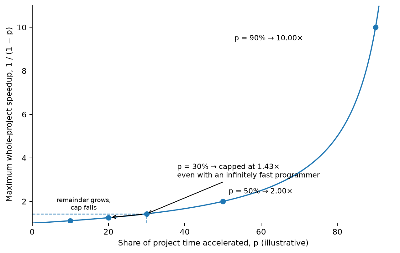
Amdahl’s cap, 1/(1−p), drawn from the table above: the curve is exact, the shares illustrative. At p = 30% even an infinitely fast programmer caps the project at 1.43× — and if the remainder grows, the cap falls.
Two readings fall out directly. Even if half of elapsed project time were in the accelerated fraction, making that fraction infinitely fast would only double the whole project under Amdahl’s assumptions. And if the intervention itself enlarges review, integration, or coordination, then the original value of p no longer describes the new process; the simple bound has to be recomputed rather than treated as a fixed law.
That resolves one part of the puzzle: 100× faster at one activity does not imply 100× faster end to end. The missing quantity is the measured share of elapsed work the intervention actually accelerates.
The same accounting intuition appears in Chapter 28’s cost experiment. Under a declared scenario of $5 for every question put to a person, its two forty-item arms differed by roughly sixfold in known model spend — about half a cent versus about three cents — while total scenario costs were $35.01 and $45.03. The dollar difference was dominated by two fewer human escalations, not by the cents of model spend. That is a measured composition result for that workload, not an estimate of software-project time shares.
DORA and GitClear motivate another question: does faster generation enlarge downstream work? DORA finds higher AI adoption associated with worse delivery stability in both 2024 and 2025, while GitClear reports more churn and duplication alongside less refactoring. Those results are compatible with additional downstream work, but neither study isolates “faster generation” as the cause or measures a growing serial fraction. The 2025 DORA throughput increase is exactly why the claim should stay at that level.
Some of the serial remainder maps directly onto responsibilities this book has already named:
| Work in the remainder | Chapter 2’s name where applicable |
|---|---|
| Deciding what should be built, and what done means | Intent |
| Deciding which effects are permitted | Authority |
| Establishing that the resulting state satisfies the required property | Verification |
| Deciding whether a model call is the right mechanism | Frontier judgment |
| Waiting, integration, coordination, deployment, and other project work | Outside this four-part vocabulary |
Chapter 2 keeps the first four responsibilities outside the generator. It does not establish that they constitute 70% of project time, that generation was never the bottleneck, or that they cannot themselves be partly automated. The practical claim is enough: if a meaningful share of elapsed time sits outside generation, improving generation alone will eventually run into that remainder.
Contemporary vendor evidence is compatible with that bottleneck shift. In September 2026 OpenAI reported that by mid-August its research organization was consuming an estimated 3.1 agent-workdays for every human workday, with the median researcher using over $600/day of inference at API prices; researchers wrote more code and ran more experiments, and OpenAI noted that the least automatable tasks take a larger share of researcher effort as other work is automated (OpenAI, 2026).
Bound it as the source demands: internal self-report, correlational, with compute also growing, and no decomposition of whole-project completion time. It supports the possibility that bottlenecks move as one component accelerates. It does not tell us which remainder dominates or how large it is.
That is still enough to motivate the next five parts. Intent, authority, state, and verification are places where end-to-end leverage can be lost even when generation gets dramatically better.
Electric motors on steam-age shafts
Amdahl says where the time goes. It does not say why it stays there. For that, economic history has a precedent close enough to be uncomfortable.
In 1990 Paul David asked why computers were not showing up in the productivity statistics, and answered with the dynamo. The first central power stations opened in the early 1880s. Electricity did not register in US manufacturing productivity until the early 1920s — four decades later, when only slightly more than half of factory mechanical drive had been electrified (David, 1990).
Part of the delay was layout. From the mid-1890s to the eve of the 1920s, factories that electrified mostly used group drive: electric motors turning sections of the same overhead shafts and belts the steam engine had turned, in buildings shaped around those shafts. Many were several stories tall, because very long line shafts wasted power. The new power source went into the old arrangement.
The large gains came with unit drive — a motor on each machine — which let the shafting and its heavy bracing go, let factories be built on a single story, and let machines be placed around the flow of materials and rearranged when the product changed.
Now look at how most people use AI. A chat window is a motor bolted onto the old shaft. The work is still arranged around a person: one request at a time, results carried by hand back into a workflow designed for human-speed generation, with the checks, the records and the decisions exactly where they were. The motorcar had a version of the same problem. Its first name was horseless carriage, and for years it looked like one.
That gives explanation two its mechanism and joins it to explanation three. Amdahl shows that the unaccelerated remainder dominates. The layout explains why the remainder does not shrink: nobody has rearranged the work so that intent is written down once, checks run without a person carrying each result to them, and every attempt leaves a record that later attempts can use. Software had been keeping exactly those books for decades, as Chapter 4 showed. A hundred geniuses in a building laid out for one typist will mostly queue.
Bound the analogy the way David bounded his. History does not repeat on schedule, and a four-decade lag for electricity says nothing precise about AI. What transfers is the mechanism: the gains arrive when the work is reorganized around the new capability, not when the capability is installed.
The respectable version of “too early”
There is a serious economic explanation that is neither “it’s fake” nor “you’re holding it wrong”, and it deserves its place.
Brynjolfsson, Rock, and Syverson gave David’s observation a measured form. They showed that general purpose technologies require large complementary intangible investments — process redesign, new skills, reorganized workflows — and that these investments are costly, take years, and are poorly captured in national accounts. The result is a J-curve: measured productivity looks flat or worse during the investment period, then rises as the intangibles pay off. Adjusting for intangibles related to computer hardware and software put total factor productivity 15.9% higher than official measures by the end of 2017 (Brynjolfsson, Rock & Syverson, 2021).
The J-curve offers a serious hypothesis for part of what current AI measurements may be missing: productivity can lag capability while organizations invest in complementary process redesign, skills, and infrastructure. The evidence in this chapter does not identify missing complements as the cause of today’s mixed AI productivity results, so the historical mechanism should not be promoted into that conclusion.
And do not read the J-curve as “wait and it will come.” The complement is work someone has to do: redesign the process, build measurement, restructure decisions, and decide where the model belongs. The analogy predicts no timetable and guarantees no payoff. It simply explains why installing a general-purpose technology and reorganizing around it are different economic events.
Scope can consume the gain
One more mechanism belongs on the list, but this chapter has not measured its size.
When capacity gets cheaper, an organization can spend the gain in several ways: finish the same scope sooner, increase quality, attempt more experiments, or expand scope. If scope expands at roughly the rate generation gets cheaper, completion time may barely move even though capability is being used productively. That is a rebound effect, not evidence by itself of either success or failure.
The stronger claims about organizational incentives — that budgets prefer ongoing work, or that capacity exhaustion historically forced most projects to close — would require evidence this chapter does not have. Keep the design consequence without pretending to have measured the motive.
If completion is the objective, something explicit has to define it. Write down what done means in advance, distinguish scope changes from work required to reach the frozen target, and record when the target moves. That is Chapter 4’s acceptance-criteria discipline promoted from task scale to project scale.
The same discipline helps with tools you build for yourself. A personal tool can legitimately keep evolving, but then “finished” must attach to bounded increments rather than to the existence of the product as a whole. Chapter 30 turns that into a measured improvement loop.
Where to look for the finished projects
If the mechanism is layout, the finished projects will not show up first as a wave of closed tickets inside processes nobody rearranged. They will show up where someone rebuilt the work around the capability. One place is domains with cheap automated checks, as AlphaEvolve showed. The other is work small enough for one person or one team to rearrange without permission from anyone else.
Chapter 30 argues that much of the second kind will look like software built around a particular person’s way of working: tools that finish the recurring jobs they were built for, one at a time, in a thousand different shapes. That would not be visible from orbit, and it would not look like a wave. It is an argument, not a measurement, and it is where this book’s own construction points.
There may also be a further drag on genuinely novel work, stated here as a hypothesis only. Where a project departs from convention, missing local context lets assistants repeatedly reintroduce the conventional solution the project rejected. Chapter 9 examines that mechanism. This chapter does not measure its contribution to completion rates.
Measure arrival, not motion
The actionable version of this chapter is short.
Many popular AI metrics measure activity: tokens, suggestions accepted, lines written, pull requests opened. Delivery programs such as DORA also measure outcomes such as throughput and instability. What is often still missing is an explicit project-level definition of arrival tied to the scope you meant to finish.
So instrument that outcome directly:
- Started versus finished, per quarter, with “finished” defined in writing before the work begins.
- Cycle time to finished, using the same definition — for example, closed and not reopened or reverted within a declared observation window.
- Rework rate: what fraction of supposedly finished work is revisited within that window.
- Backlog age and scope change: distinguish old work that is not closing from new work intentionally added to the target.
These are Chapter 7’s measurement discipline applied one level up: define the outcome first, preserve item-level history, and do not let a proxy such as lines written stand in for the thing you actually care about.
Do this now
Thirty minutes with your issue tracker. Count arrivals as well as motion.
- Choose one bounded class of work for which “finished” can be stated consistently. For the last four quarters, count items started and items finished using that rule — for example, closed and not reopened or reverted within thirty days.
- Plot the ratio. Mark when AI tooling changed, but label that marker as context, not as a causal intervention by itself.
- Compute the same measures for the preceding period if the records are comparable. Also record obvious changes in team size, scope policy, release process, or work mix that could move the ratio.
- Separately, estimate what fraction p of elapsed time the AI intervention could plausibly accelerate. Compute
1 / (1 - p)as an illustrative upper bound under Amdahl’s assumptions, not as a measured explanation of your observed result. - Find one shaft. Name a place where AI output reaches the work only because a person carries it there. Write down what check could run automatically, what state would have to be preserved, and what evidence each attempt should leave.
Now compare the observations. If arrival improved, you have a result worth investigating. If it did not, you have hypotheses — an accelerated fraction that was too small, downstream work that grew, scope expansion, weak measurement, or something else — not a causal diagnosis yet.
Bring that distinction, not just the ratio, to whoever is budgeting your AI spend.
Failure modes
- Measuring motion and calling it productivity. Tokens, suggestions, and drafts all rise while completions do not.
- Expecting linear speedup from a nonlinear system. Amdahl caps you well below the coworker’s individual multiplier.
- Ignoring that acceleration enlarges the unaccelerated part. More generated code means more review and integration surface.
- Treating churn as neutral. Churn is work redone. A rising churn rate is the signature of a project moving away from done.
- Quoting one year of DORA. The 2024 and 2025 findings differ; the stability finding is what persists.
- Reading the J-curve as permission to wait. The complementary investment is the work, and somebody has to do it.
- Bolting the motor onto the old shaft. A chat window added to an unchanged process leaves every check, record and decision where it was.
- Reading the missing wave as proof the capability is fake. Finished results exist where the process was built around a cheap check.
- Assuming everyone wants closure. Removing the capacity constraint removes the main historical reason things ended.
What this chapter established
- Large capability claims create a measurable question: does bounded work reach its defined terminal state sooner or more often? This chapter does not have an industry-wide started-versus-finished measure, so absence of that measure is a limitation, not evidence of absent completion.
- AlphaEvolve supplies a concrete positive case for the checkability thesis: model proposals were searched under automated evaluators and produced objectively improved algorithms on selected problems. It does not establish that the same conditions explain ordinary project completion.
- The adjacent evidence is mixed: DORA associates higher AI adoption with worse delivery stability in both 2024 and 2025 while throughput changes sign; METR’s early slowdown was later qualified by a selection-limited update; GitClear reports more churn and duplication and less refactoring without establishing AI causation.
- Amdahl’s law gives a conditional bound. If 30% of elapsed work were the accelerated fraction and the remaining 70% were unaffected, making that fraction infinitely fast would cap whole-project speedup at 1.43×. The 30/70 split is illustrative, not measured.
- Intent, authority, verification, and frontier judgment are important parts of some serial remainders, but Chapter 2 does not establish that they constitute the whole remainder or a fixed share of project time. Integration, waiting, coordination, deployment, and other work remain too.
- The electricity analogy supplies a mechanism worth testing: a general-purpose technology can require complementary process redesign before its capability appears as system-level productivity. It is an analogy, not a forecast for AI.
- The J-curve literature shows that complementary intangible investment can delay measured productivity gains from general-purpose technologies. It does not establish that missing complements explain today’s mixed AI results.
- Scope expansion is another plausible mechanism: cheaper capacity can be spent on more ambition rather than earlier completion. This chapter treats that as a design risk, not a measured organizational law.
- Measure arrival directly: started versus finished under a frozen definition, cycle time to that state, rework within a declared window, backlog age, and scope changes.
Next
Part 1 is done. It has been argument, because the arguments determine what is worth building: where to stand, which operations may be stochastic, which terrain repays effort, what keeps the reviewer honest, what it all costs, how you would know if it worked, and which parts of the process can constrain completion.
That is enough to decide the shape of what follows. If generation is only one component of completion, a runtime for AI work cannot be just a wrapper around a model. It needs explicit intent, durable state, enforceable authority, and verification whose evidence survives the call.
So the next chapter stops arguing and states the system: one that works wherever you happen to be, never loses context, remembers everything it has done, reaches for the best cheapest model it can actually get, and reviews every contribution it makes. Five properties — each one forced by an argument in Part 1, and each one in tension with at least one of the others.
Continue with One Runtime, Many Windows.
References
- Dario Amodei. Machines of Loving Grace: How AI Could Transform the World for the Better. October 2024. https://www.darioamodei.com/essay/machines-of-loving-grace — describes a hypothetical future system, not a deployed one.
- Alexander Novikov et al. (Google DeepMind). AlphaEvolve: A Coding Agent for Scientific and Algorithmic Discovery. arXiv:2506.13131, June 2025. https://arxiv.org/abs/2506.13131
- Paul A. David. The Dynamo and the Computer: An Historical Perspective on the Modern Productivity Paradox. American Economic Review, vol. 80, no. 2 (1990), pp. 355–361. https://ideas.repec.org/a/aea/aecrev/v80y1990i2p355-61.html
- DORA / Google Cloud. Accelerate State of DevOps Report 2024. https://dora.dev/research/2024/dora-report/
- DORA / Google Cloud. Announcing the 2025 DORA Report. https://cloud.google.com/blog/products/ai-machine-learning/announcing-the-2025-dora-report
- Joel Becker, Nate Rush, Elizabeth Barnes, and David Rein (METR). Measuring the Impact of Early-2025 AI on Experienced Open-Source Developer Productivity. arXiv:2507.09089, 2025. https://arxiv.org/abs/2507.09089
- Erik Brynjolfsson, Daniel Rock, and Chad Syverson. The Productivity J-Curve: How Intangibles Complement General Purpose Technologies. American Economic Journal: Macroeconomics, vol. 13, no. 1 (2021), pp. 333–372. https://doi.org/10.1257/mac.20180386
- GitClear. AI Copilot Code Quality: 2025 Data Suggests Downward Pressure on Code Quality. Vendor research; not peer-reviewed. https://www.gitclear.com/ai_assistant_code_quality_2025_research
- Gene M. Amdahl. Validity of the Single Processor Approach to Achieving Large Scale Computing Capabilities. AFIPS Spring Joint Computer Conference, 1967, pp. 483–485. https://doi.org/10.1145/1465482.1465560
- OpenAI. Research acceleration: The view inside OpenAI. 6 September 2026. https://openai.com/index/research-acceleration-view-inside-openai/ — Vendor self-report of internal usage; correlational.