Encode All 256 Elementary Rules
In the previous chapter we built one rule: a cell becomes active when exactly one of its three neighbors is active. That turned out to be Rule 22, but we treated it as a hand-written function.
Now we generalize. Instead of writing one function per rule, we encode every possible elementary rule as a single integer — and get all 256 automata for the price of one simulator.
An elementary cellular automaton has only three inputs per cell:
left centre right
Each input is one bit.
That means there are only eight possible neighborhoods:
111 110 101 100 011 010 001 000
For each neighborhood the rule chooses either 0 or 1.
Eight binary choices means:
2^8 = 256
possible rules.
The elegant part is that we can store one complete rule table in one byte.
This enumeration goes back to Wolfram’s systematic survey of the one-dimensional rules in the early 1980s: same grid, same neighborhoods, every table tried in turn. The number is the table.
Rule numbers are lookup tables
Take Rule 30.
Thirty in eight-bit binary is:
00011110
Read those bits against the neighborhoods in descending order, with 111 as the most significant bit:
| Neighborhood | Output |
|---|---|
| 111 | 0 |
| 110 | 0 |
| 101 | 0 |
| 100 | 1 |
| 011 | 1 |
| 010 | 1 |
| 001 | 1 |
| 000 | 0 |
So the rule number is not a mysterious label.
It is the transition table encoded as an integer.
The ordering convention is what makes the number meaningful: 111 first, 000 last, bits read left to right as an eight-bit value. Any consistent ordering would work, but this descending order is the shared convention, so 00000010 unambiguously means Rule 2 — only neighborhood 001 produces a live cell.
    flowchart LR
    A[Rule number] --> B[8-bit binary table]
    B --> C[Neighborhood outputs]
    C --> D[Shared local transition]
One qualification worth stating early: 256 labels does not mean 256 fundamentally different behaviors. Some rules are mirror images or complements of each other — reflection and state relabeling identify equivalent pairs — leaving 88 essentially distinct rules. Rule 30’s own family makes this concrete:
| Transformation | Rule | Relation to Rule 30 |
|---|---|---|
| none | 30 | 00011110 |
| mirror image | 86 | left-right reflection |
| complement | 135 | 0 and 1 exchanged |
| mirror complement | 149 | both at once |
The number is an address, not a complexity ranking. Which addresses are interesting is an empirical question, and the rest of Part I answers it rule by rule.
More generally, the counting argument scales: a deterministic rule with k states and n neighborhood sites has k^n possible local inputs and k^(k^n) possible tables. The elementary setting (k = 2, n = 3) is simply the smallest case where that space is both fully enumerable and surprisingly rich.
Turn a neighborhood into an index
A three-bit neighborhood already has a natural integer value:
000 -> 0
001 -> 1
010 -> 2
011 -> 3
100 -> 4
101 -> 5
110 -> 6
111 -> 7
We can compute that without strings:
def neighborhood_index(left, centre, right):
    return (left << 2) | (centre << 1) | right
Then extract the corresponding bit from the rule number:
def elementary_rule(rule_number, left, centre, right):
    index = neighborhood_index(left, centre, right)
    return (rule_number >> index) & 1
That one function can execute any elementary rule from 0 to 255.
There is a useful consistency check here. For Rule 30, neighborhood 100 has index 4, so:
(30 >> 4) & 1 = 1
which matches the table above. And our Rule 22 from the previous chapter falls out the same way: neighborhoods 100, 010, 001 have indices 4, 2, 1, so bits 4, 2, and 1 are set — 16 + 4 + 2 = 22, or 00010110. The hand-written local_rule and elementary_rule(22, ...) agree on all eight inputs.
A complete simulator
Unlike the previous chapter’s run, which accepts any rule function and any
initial state, this version specializes to the elementary setting: it takes a
rule number and builds the single-cell start itself. (The next chapter
generalizes back with run_from_state.)
import numpy as np


def step(state, rule_number):
    next_state = np.zeros_like(state)

    for i in range(len(state)):
        left = state[(i - 1) % len(state)]
        centre = state[i]
        right = state[(i + 1) % len(state)]
        next_state[i] = elementary_rule(
            rule_number, left, centre, right
        )

    return next_state


def run(rule_number, width=101, generations=100):
    state = np.zeros(width, dtype=np.uint8)
    state[width // 2] = 1

    history = [state.copy()]

    for _ in range(generations - 1):
        state = step(state, rule_number)
        history.append(state.copy())

    return np.array(history)
Now exploring a different automaton is just:
history = run(30)
or:
history = run(110)
or:
history = run(184)
The engine stays fixed.
Only the local law changes.
Note what step assumes, carried over from the previous chapter: synchronous parallel update on a periodic ring. The encoding changes the rule; it does not change the update scheme or the boundary.
Generate every rule
import matplotlib.pyplot as plt

fig, axes = plt.subplots(16, 16, figsize=(16, 16))

for rule_number, ax in enumerate(axes.flat):
    history = run(rule_number, width=63, generations=40)
    ax.imshow(history, cmap="binary", interpolation="nearest")
    ax.set_title(str(rule_number), fontsize=6)
    ax.axis("off")

plt.tight_layout()
plt.show()
The book’s reproducible figure script generates the same experiment as a canonical asset:
python scripts/figures/cellular-automata/part01_foundations.py 02
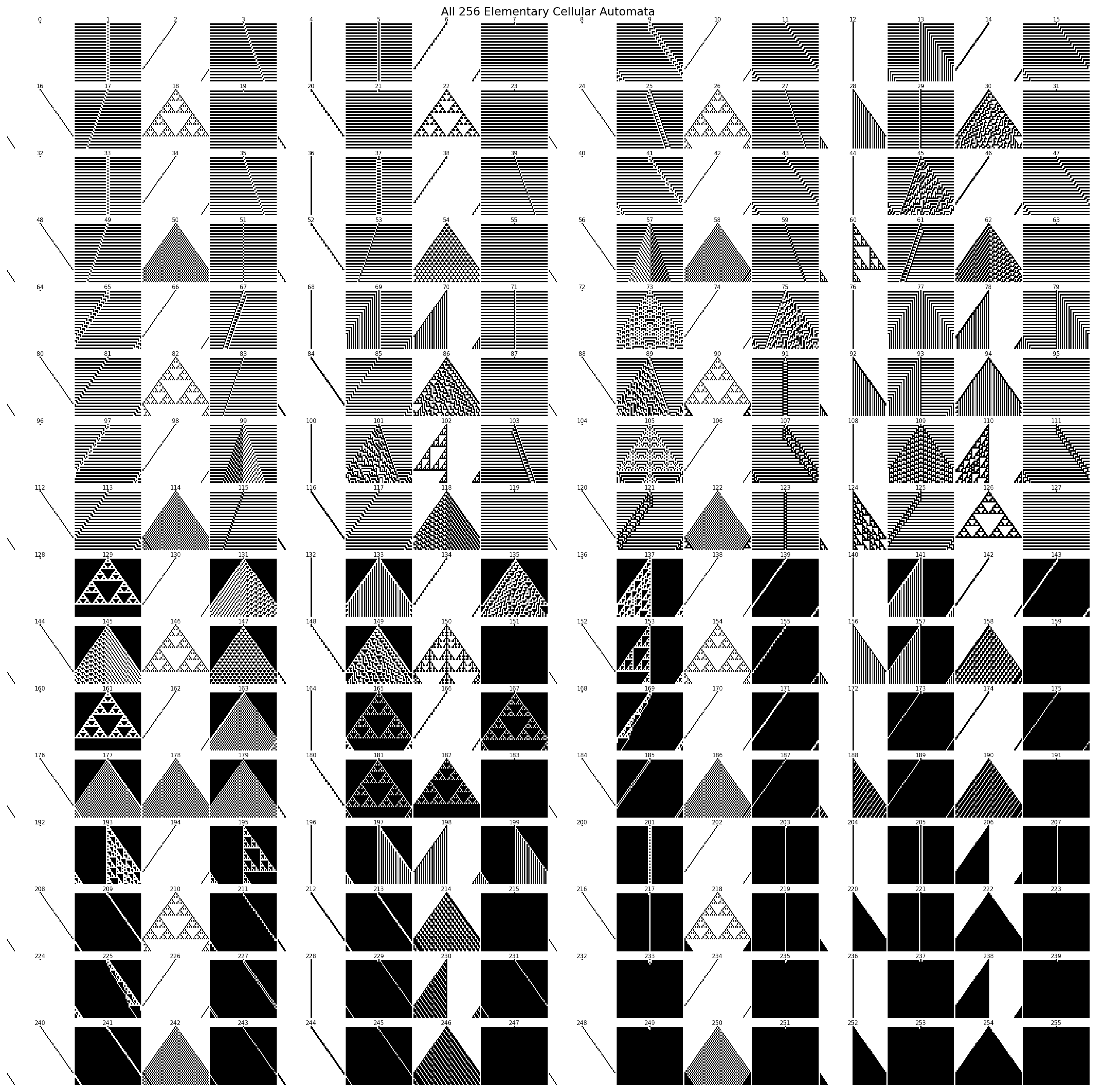
This is one of the best experiments in the subject.
The rules have exactly the same:
- grid,
- state space,
- neighborhood,
- initial condition,
- execution engine.
Only eight output bits differ.
Yet the resulting systems look radically different.
That is emergence in a form we can inspect directly — with the caveat from Chapter 1: most of those 256 panels are dull. A few are remarkable. The encoding lets us find out which.
Compare rules by measurements, not just pictures
A visual catalog is useful, but we can also measure the histories. These are deliberately crude first instruments — Chapters 18–20 will formalize measurement — but they establish the habit early: replace “looks complicated” with an observable.
Density
def density_curve(history):
    return history.mean(axis=1)
(Named to match Chapter 18’s formal owner — these previews use the curve forms throughout.)
This tells us what fraction of cells are active at each generation.
Change rate
def change_curve(history):
    return np.mean(history[1:] != history[:-1], axis=1)
This measures how much each generation differs from the previous one.
Spatial entropy
For a binary row with active-cell probability p:
import numpy as np


def binary_entropy(row):
    p = row.mean()
    if p in (0.0, 1.0):
        return 0.0
    return -(p * np.log2(p) + (1 - p) * np.log2(1 - p))
This quantity measures the balance between zeros and ones in one row. It does not by itself measure spatial organization: two rows with the same density have the same binary entropy even if one contains long blocks and the other alternates rapidly.
That limitation is useful. It teaches us to ask what a metric actually observes rather than giving a number more meaning than it has.
These are crude measurements, but they change the question from:
Which rule looks complicated?
to:
Which observable properties distinguish one dynamical regime from another?
That is a much stronger habit.
Initial conditions matter too
A single central cell is convenient, but it is not the whole story.
Try a random state:
rng = np.random.default_rng(42)
state = rng.integers(0, 2, size=101, dtype=np.uint8)
Or a repeating pattern:
state = np.resize(np.array([1, 0, 0], dtype=np.uint8), 101)
A cellular automaton is a dynamical system.
The behavior belongs to the combination:
rule + initial state + boundary conditions + update scheme
not to the rule number alone.
The important abstraction
We can now separate the system into three pieces:
encoding
  rule number -> transition table

runtime
  neighborhood -> update -> next generation

experiment
  initial state + duration + measurements
That is already enough to build a serious exploration tool.
In the next chapter we will focus on one of the most famous rules in the catalog: Rule 30.
Its local rule is tiny.
Its global pattern looks anything but tiny.
Research
Wolfram, S. — Statistical Mechanics of Cellular Automata (Reviews of Modern Physics 55, 1983). Origin of the enumeration this chapter implements: all one-dimensional binary nearest-neighbor tables, surveyed with the same grid, neighborhoods, and initial conditions while only the output bits vary. Read the setup, not just the classification. https://doi.org/10.1103/RevModPhys.55.601
Weisstein, E. W. — Elementary Cellular Automaton (MathWorld). The encoding reference: 8 neighborhoods,
2^8 = 256rules indexed by an 8-bit number, with Rule 30/90/110 as worked Boolean forms — plus the 88-fundamentally-inequivalent count under reflection and complementation used for this chapter’s qualification. https://mathworld.wolfram.com/ElementaryCellularAutomaton.htmlZenil, H. & Martinez, G. J. — Cellular Automata (Scholarpedia). States the naming convention precisely (outputs ordered
111down to000read as binary;00000010is Rule 2) and gives the general counting law (k^ninputs,k^(k^n)tables). Use it to check any rule-decoding code against an independent statement of the convention. http://www.scholarpedia.org/article/Cellular_automataBerto, F. & Tagliabue, J. — Cellular Automata (Stanford Encyclopedia of Philosophy). Corroborates the convention with a second worked example (Rule 90 as
01011010) and places the 256-rule survey inside Wolfram’s four-class taxonomy, which the next chapters will use and qualify. https://plato.stanford.edu/entries/cellular-automata/