Build a Forest Fire Simulation

The previous chapter put probability into the rule. A forest fire is almost an ideal first exercise for using it.

The visible states are obvious:

0 = empty
1 = tree
2 = burning

The interactions are local.

And small changes in fuel density or ignition assumptions can produce very different global outcomes.

This is not intended as a high-fidelity wildfire model.

It is a deliberately simplified spread model designed to isolate one mechanism:

How does local fuel connectivity determine whether fire propagates through a landscape?

That isolation is a deliberate subtraction from the classic Drossel–Schwabl forest-fire model (1992), whose four synchronous processes are tree growth with probability p, spontaneous ignition with probability f, spread from burning neighbors, and burning-to-empty. This chapter keeps spread plus optional lightning, uses the eight-cell Moore neighborhood rather than the original four-cell one, fixes the forest instead of regrowing it, and studies one fire — so that connectivity, not the full growth–burn cycle, is what varies. The regrowth section at the end reconnects the two.

Initialize the forest

import numpy as np

EMPTY = 0
TREE = 1
FIRE = 2


def make_forest(
    rows=150,
    cols=200,
    tree_density=0.65,
    seed=42,
):
    rng = np.random.default_rng(seed)

    grid = np.zeros(
        (rows, cols),
        dtype=np.uint8,
    )

    grid[
        rng.random((rows, cols)) < tree_density
    ] = TREE

    return grid

Ignite one cell:

forest = make_forest()

forest[
    forest.shape[0] // 2,
    forest.shape[1] // 2,
] = FIRE

Now tree_density becomes an experimental parameter.

At low density, burning regions may encounter gaps.

At high density, the tree network may become connected enough for fire to travel much farther.

Both are hedged on purpose: whether fire percolates is an outcome of the density and the realization, which is why the chapter ends in distributions rather than verdicts.

Detect burning neighbors without wraparound

For a literal forest map, the left edge should not normally touch the right edge.

That means periodic np.roll boundaries would create a modeling artifact.

A useful helper is a fixed-edge shift:

def shift_fixed(a, dy, dx):
    out = np.zeros_like(a)

    src_y0 = max(0, -dy)
    src_y1 = a.shape[0] - max(0, dy)
    src_x0 = max(0, -dx)
    src_x1 = a.shape[1] - max(0, dx)

    dst_y0 = max(0, dy)
    dst_y1 = a.shape[0] - max(0, -dy)
    dst_x0 = max(0, dx)
    dst_x1 = a.shape[1] - max(0, -dx)

    out[
        dst_y0:dst_y1,
        dst_x0:dst_x1,
    ] = a[
        src_y0:src_y1,
        src_x0:src_x1,
    ]

    return out

(Verified: shifting a test grid down one row reproduces the top rows exactly with a zeroed top edge.)

Then:

def burning_neighbor_mask(grid):
    burning = grid == FIRE
    near_fire = np.zeros_like(
        burning,
        dtype=bool,
    )

    for dy in (-1, 0, 1):
        for dx in (-1, 0, 1):
            if dy == 0 and dx == 0:
                continue

            near_fire |= shift_fixed(
                burning,
                dy,
                dx,
            )

    return near_fire

Boundary behavior is part of the model, so it should be visible in the implementation. This is the fixed-boundary case from the boundary taxonomy: exterior values are treated as non-burning, stated in code rather than left implicit.

Write one synchronous update

def forest_step(
    grid,
    rng,
    lightning_probability=0.0,
):
    next_grid = grid.copy()

    burning = grid == FIRE
    trees = grid == TREE
    near_fire = burning_neighbor_mask(grid)

    next_grid[burning] = EMPTY

    ignite_from_neighbor = trees & near_fire

    lightning = (
        trees
        & (
            rng.random(grid.shape)
            < lightning_probability
        )
    )

    next_grid[
        ignite_from_neighbor | lightning
    ] = FIRE

    return next_grid

Each transition remains readable:

    flowchart LR
    B[burning] --> E[empty]
    T[tree] --> BN{burning neighbor?}
    BN -->|yes| F[burning]
    T --> L{lightning draw?}
    L -->|yes| F
    BN -->|no| T2[stays tree]
    L -->|no| T2
    E2[empty] --> E2
  

burning -> empty

tree + burning neighbor -> burning

tree + lightning event -> burning

Note the two ignition paths from the previous chapter’s taxonomy: neighbor-conditioned spread (deterministic here) and independent spontaneous ignition (probability lightning_probability). Same generator, different causal models — kept visibly separate.

That readability matters more than compressing the entire rule into one expression.

Run until the fire dies out

def run_fire(
    initial,
    steps=250,
    seed=123,
    lightning_probability=0.0,
):
    rng = np.random.default_rng(seed)
    grid = initial.copy()
    history = []

    for _ in range(steps):
        history.append(grid.copy())

        if (
            not np.any(grid == FIRE)
            and lightning_probability == 0
        ):
            break

        grid = forest_step(
            grid,
            rng,
            lightning_probability,
        )

    return np.array(history)

With spontaneous ignition disabled:

no burning cells
      ->
no future burning cells

That is a useful termination invariant.

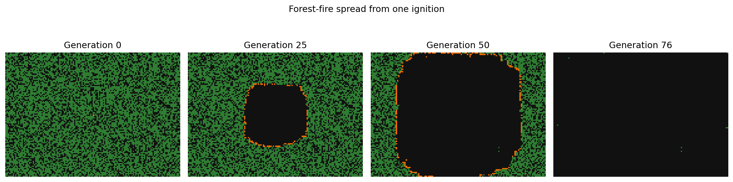
(Verified on a 40×50 test forest at density 0.65: the fire terminates after 30 recorded states with effectively the whole initial fuel load consumed — one realization, not a claim about all densities.)

Measure the state populations

The animation tells us where the fire moved.

Population curves tell us what the process did overall.

def state_counts(grid):
    return {
        "empty": int(
            np.count_nonzero(grid == EMPTY)
        ),
        "trees": int(
            np.count_nonzero(grid == TREE)
        ),
        "burning": int(
            np.count_nonzero(grid == FIRE)
        ),
    }

Collect that every generation.

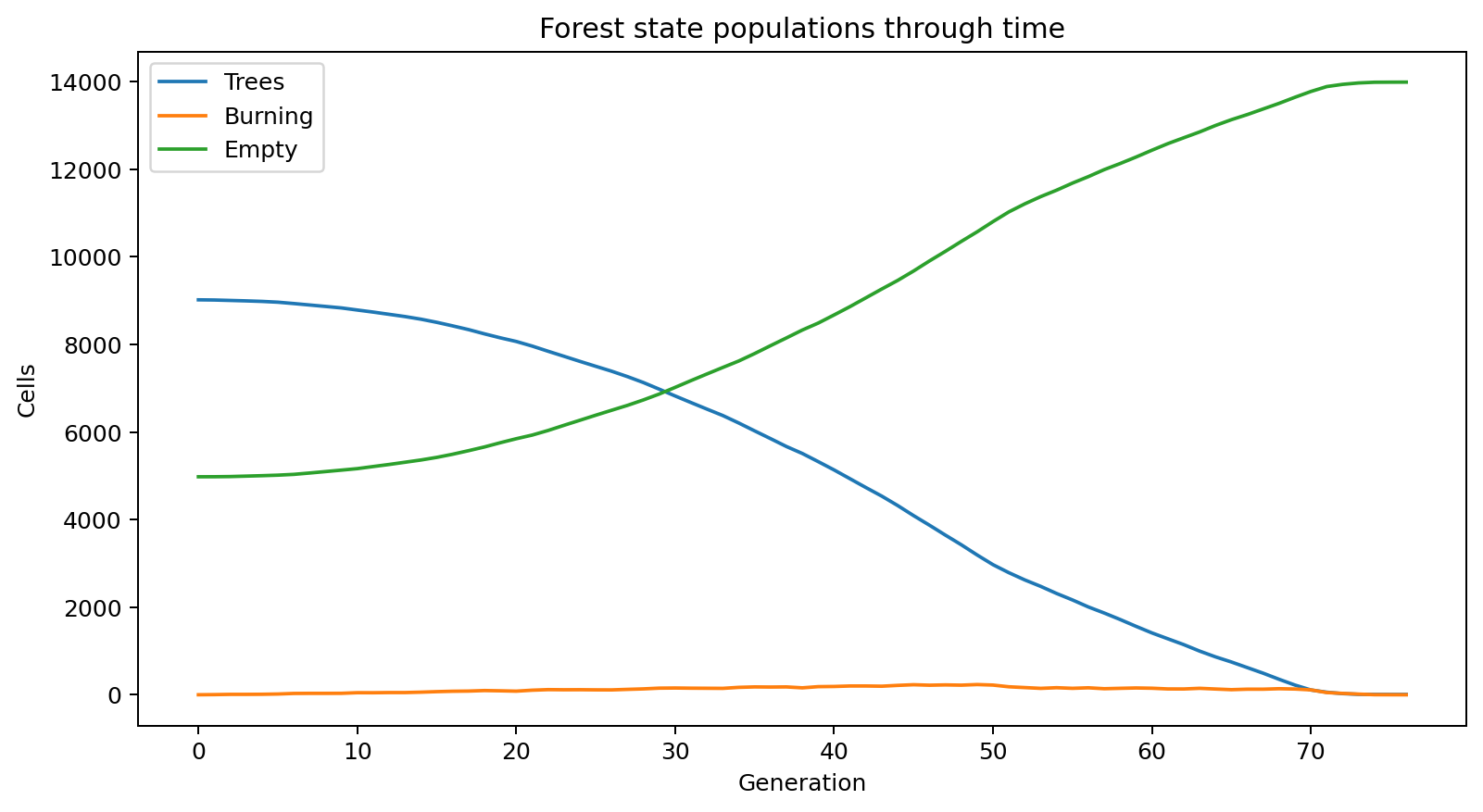
The burning population rises while connected fuel is available, then collapses as the local front runs out of reachable trees.

Measure burn fraction

def fire_summary(initial, final):
    initial_trees = np.count_nonzero(
        initial == TREE
    )

    surviving_trees = np.count_nonzero(
        final == TREE
    )

    burned = initial_trees - surviving_trees

    return {
        "initial_trees": int(initial_trees),
        "surviving_trees": int(
            surviving_trees
        ),
        "burned": int(burned),
        "burn_fraction": (
            burned / initial_trees
            if initial_trees
            else 0.0
        ),
    }

Now sweep density across many seeds.

That experiment is more informative than selecting one dramatic animation.

We can ask:

At density d,
what is the distribution of burn fractions?

That question separates a stochastic realization from a model-level claim — the exact discipline the previous chapter introduced.

Add direction only when the mechanism demands it

The current model treats all neighboring directions equally.

A wind-biased model would not.

Conceptually:

burning neighbor west of tree
    -> higher ignition probability

burning neighbor east of tree
    -> lower ignition probability

That changes the neighborhood from an unordered collection into a directional one.

The general lesson is:

An anisotropic world requires an anisotropic local rule.

Do not add wind as a cosmetic animation effect. Put it into the transition probabilities.

Add regrowth to create a persistent system

If empty cells can regrow trees and trees can ignite spontaneously, the world no longer terminates.

A slow regrowth process can compete with a fast burning process:

slow:
trees accumulate
      ↓
fuel network forms

fast:
ignition occurs
      ↓
fire consumes connected fuel

The interaction between timescales can generate long-running global dynamics.

This is the doorway back to Drossel–Schwabl: with separated timescales — regrowth much faster than the wait between lightning strikes — they proposed the system organizes to a critical state with power-law fire sizes (“self-organized criticality”). Treat that as a proposed interpretation of a fuller model, not as something this chapter’s single-fire experiments establish. Testing it would require the regrowth–lightning apparatus, long steady-state runs, and scaling analysis — a project, not a paragraph.

One idea to keep

This chapter is not valuable because it looks like a fire.

It is valuable because we can state exactly what the model contains:

space
state
neighborhood
boundary condition
spread rule
random process
initial fuel density

and then ask how changing one ingredient alters the outcome distribution.

In the next chapter we will use the same local viewpoint for a conserved moving quantity: cars on a one-dimensional road, governed by Rule 184.

Research

• Drossel, B. & Schwabl, F. — Self-organized critical forest-fire model (Physical Review Letters 69, 1992). The classic reference this chapter subtracts from: three states (tree, burning, empty) with four synchronous processes — growth p, lightning f, neighbor spread, burning-to-empty — on a von Neumann neighborhood, with criticality proposed in the f → 0 timescale-separated limit. Read it to see exactly which mechanisms this chapter fixed or removed, and what would need restoring (regrowth, steady state, scaling analysis) before any criticality claim. The link below is a university course project that explains the model, not the paper itself; check the original before quoting it. https://itp.uni-frankfurt.de/~gros/StudentProjects/Projects_2020/projekt_lars_dingeldein/

• Zenil, H. & Martinez, G. J. — Cellular Automata (Scholarpedia). The caution that governs this chapter’s modesty: visually plausible patterns are not by themselves evidence that a model describes a natural system, and domain applications add assumptions that require comparison with observations. Applies directly to every “looks like a fire” temptation. http://www.scholarpedia.org/article/Cellular_automata

• Berto, F. & Tagliabue, J. — Cellular Automata (Stanford Encyclopedia of Philosophy). Places the spread model in the applications lineage (discrete dynamical-system simulators for physical and biological processes) and restates the contract this chapter implements: probabilities belong to the rule, realizations vary. https://plato.stanford.edu/entries/cellular-automata/