Diffusion as Local Exchange
Until now most cells have stored discrete state:
0 / 1
empty / tree / fire
road / car
Now let each cell store a continuous quantity.
For diffusion:
state[y, x] = concentration
The local transition is no longer birth, death or movement.
It is local exchange.
This steps outside the strict finite-state definition — a deliberate extension, flagged as such, that the book will keep developing through reaction-diffusion, Lenia, and learned automata.
Start with a pulse
import numpy as np

size = 121

grid = np.zeros(
    (size, size),
    dtype=np.float64,
)

grid[
    size // 2,
    size // 2,
] = 1.0
At the beginning one cell contains all the concentration.
Repeated local exchange should spread that quantity outward.
The discrete Laplacian
A four-neighbor periodic Laplacian is:
def laplacian(grid):
    return (
        np.roll(grid, 1, axis=0)
        + np.roll(grid, -1, axis=0)
        + np.roll(grid, 1, axis=1)
        + np.roll(grid, -1, axis=1)
        - 4 * grid
    )
Interpret it locally.
If a cell is higher than its neighbors, the Laplacian tends to be negative.
If it is lower than its neighbors, the Laplacian tends to be positive.
So it tells us which way local differences should relax.
One explicit diffusion step
def diffusion_step(
    grid,
    rate=0.15,
):
    return (
        grid
        + rate * laplacian(grid)
    )
Run it:
for _ in range(120):
    grid = diffusion_step(grid)
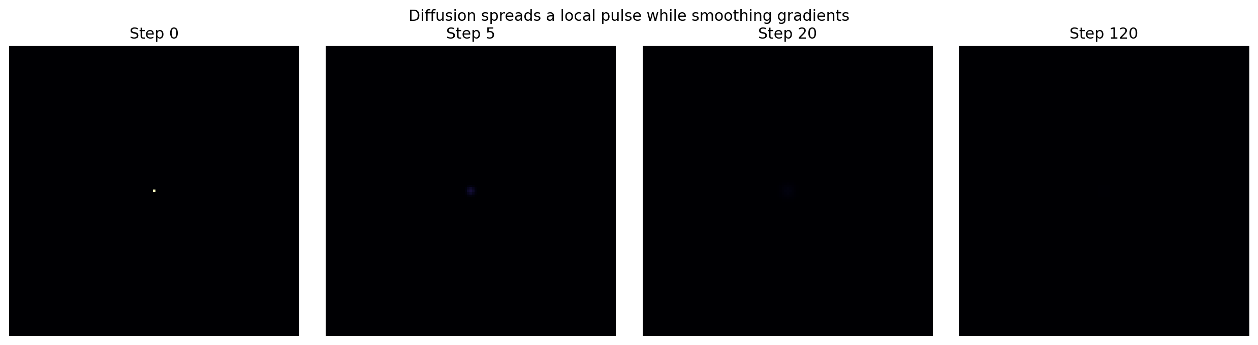
The pulse spreads without any cell knowing where the source was.
There is no global smoothing operator examining the whole map.
Every update is assembled from nearest-neighbor differences.
Conservation is the first thing to test
With periodic boundaries, the Laplacian contributions sum to zero.
So this discrete update should conserve total concentration up to floating-point error.
initial_total = grid.sum()

for _ in range(50):
    grid = diffusion_step(grid)

final_total = grid.sum()

assert np.isclose(
    initial_total,
    final_total,
)
Note isclose rather than exact equality: floating-point summation order makes bit-exact conservation the wrong test. (Verified: totals match to six decimals across all stable rates below.)
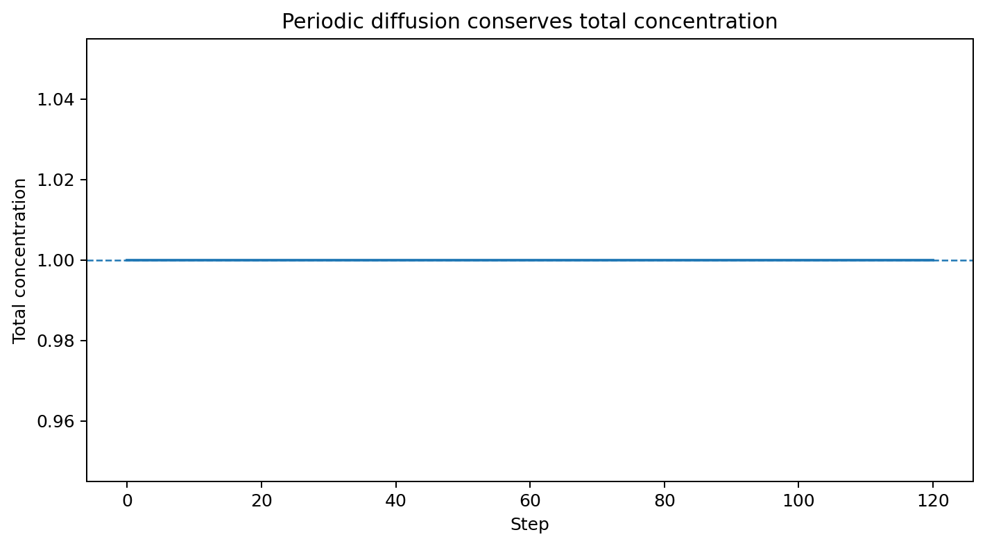
This is one reason invariants are so valuable.
A heatmap can look plausible while leaking or inventing material.
A conservation check can expose that immediately.
Why the local rule smooths differences
Consider a one-dimensional slice:
0.0 0.0 1.0 0.0 0.0
At the center:
neighbors lower
-> negative Laplacian
-> concentration falls
At adjacent cells:
one neighbor much higher
-> positive Laplacian
-> concentration rises
Repeated updates reduce local gradients.
That is the mechanism.
Numerical stability is part of the model implementation
The explicit scheme is stable only for small rates. On this four-neighbor 2D stencil the stability limit is rate ≤ 1/4: at 0.24 the pulse spreads cleanly, at 0.26 it erupts into enormous oscillating negative values (verified by direct experiment).
The stencil, its weights, and what each part contributes:
| Stencil position | Weight in laplacian | Role |
|---|---|---|
| center cell | −4 | removes local mass proportional to its own height |
| 4 axial neighbors | +1 each | collect mass from each direction |
| diagonal cells | 0 (excluded) | keeps the stencil compact and axis-aligned |
| outside the grid | wrapped (periodic) | no edge; finite-size effects instead |
A four-neighbor stencil is a modeling choice, not a law: eight-neighbor or larger stencils change both the stability limit and the isotropy of spreading.
Try an excessively large rate:
grid = diffusion_step(
    grid,
    rate=1.0,
)
The update can oscillate, produce negative values or become unstable.
Measured directly — maximum absolute concentration over 80 steps from a single-cell pulse, log scale:
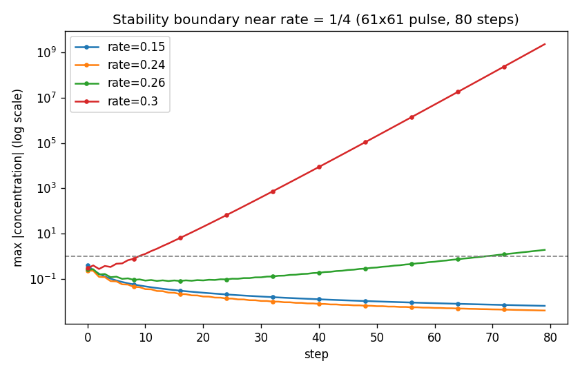
Rates 0.15 and 0.24 decay smoothly as the pulse spreads; 0.26 climbs past 1.0 and 0.30 detonates toward 10^9. The boundary is sharp and it is numerical, not physical: nothing interesting emerges above it, the discretization just stops approximating diffusion. That is the guardrail — numerical instability is a bug in the scheme, never an emergent behavior to interpret.
That teaches an important simulation lesson:
continuous equation
       !=
arbitrary discrete time step
A discrete implementation carries assumptions about spatial spacing, time step and numerical stability.
When we later build reaction-diffusion systems, those assumptions matter even more.
Measure spread directly
Instead of saying that the pulse “looks wider,” measure its second moment.
def spread_radius(grid):
    y, x = np.indices(grid.shape)
    total = grid.sum()

    cx = (x * grid).sum() / total
    cy = (y * grid).sum() / total

    r2 = (
        (x - cx) ** 2
        + (y - cy) ** 2
    )

    return np.sqrt(
        (r2 * grid).sum()
        / total
    )
Collect that through time and we get a quantitative measure of spreading — and it matches diffusion theory exactly: after 120 steps at rate 0.15 the measured radius is 8.49 against a theoretical √(4·rate·t) of 8.49. When a metric and a theory agree to two decimals, the implementation has earned trust.
The image answers:
Where is the concentration?
The metric answers:
How far has the distribution spread?
Both are useful.
Sources, sinks and obstacles change the geometry
A maintained source can keep a region at high concentration.
A sink can remove concentration.
Walls can prevent exchange across selected edges.
At that point geometry becomes part of the dynamics:
cell values
+
which neighbors can exchange
=
effective transport network
This is a recurring idea.
The grid is not merely storage.
Its connectivity determines possible causal interactions.
Continuous state opens a new design space
Conceptually we moved from:
state[y, x] = 0 or 1
to:
state[y, x] = concentration
Soon we will move again:
state[y, x] = [u, v]
and later:
state[y, x, channel]
The cell is becoming a local vector of interacting state.
One idea to keep
Pure diffusion removes local differences.
Left alone, it tends to erase structure.
So if we want persistent spots, stripes or moving boundaries, something must compete with that smoothing process — with the guardrail that a lattice analogy to a physical process is not yet a validated physical model. Resemblance is the starting point of modeling, not its conclusion.
In the next chapter we will add a local reaction to two diffusing fields and build a Gray-Scott reaction-diffusion system.
Research
Zenil, H. & Martinez, G. J. — Cellular Automata (Scholarpedia). Supplies this chapter’s two scope conditions: continuous-valued extensions (fuzzy automata and kin) lie outside the strict finite-state definition, and reaction-diffusion equations are continuous models that discrete lattices can approximate or qualitatively reproduce — a cellular-automaton analogy and a quantitatively validated approximation are different kinds of model. http://www.scholarpedia.org/article/Cellular_automata
Berto, F. & Tagliabue, J. — Cellular Automata (Stanford Encyclopedia of Philosophy). Places lattice diffusion work in the simulator lineage (discrete models of turbulence and transport reproducing continuum behavior at the macroscale) while keeping the mechanism-first framing: simple local conservation laws generating collective behavior. https://plato.stanford.edu/entries/cellular-automata/