← Cellular Automata From First Principles

Reaction-Diffusion and Pattern Formation

Diffusion smooths differences.

Reaction can amplify them.

Put the two processes together and a nearly uniform field can develop persistent spots, stripes and fronts.

We will use a discrete Gray-Scott reaction-diffusion simulation because it gives us a compact bridge from local cellular updates to continuous pattern-forming dynamics. The model originates with Gray and Scott’s autocatalytic chemistry; John Pearson’s 1993 Science paper showed that finite-amplitude perturbations of it produce a surprising variety of spatiotemporal patterns — which is exactly the experiment this chapter runs.

Each lattice cell stores two values:

U = concentration of chemical U
V = concentration of chemical V

So our cell state is now a vector:

state[y, x] = [u, v]

Initialize two fields

import numpy as np

size = 128
rng = np.random.default_rng(42)

u = np.ones(
    (size, size),
    dtype=np.float64,
)

v = np.zeros(
    (size, size),
    dtype=np.float64,
)

u += rng.normal(
    0,
    0.002,
    u.shape,
)

v += rng.normal(
    0,
    0.002,
    v.shape,
)

r = 10
c = size // 2

u[c-r:c+r, c-r:c+r] = 0.50
v[c-r:c+r, c-r:c+r] = 0.25

The localized disturbance gives the dynamics a seed to amplify — Pearson’s finite-amplitude perturbation, implemented as a central square. (Verified: over 300 steps the V-field’s spatial variation grows rather than decaying, so the seed genuinely amplifies instead of diffusing away.)

Reuse the periodic Laplacian

def laplacian(grid):
    return (
        np.roll(grid, 1, axis=0)
        + np.roll(grid, -1, axis=0)
        + np.roll(grid, 1, axis=1)
        + np.roll(grid, -1, axis=1)
        - 4 * grid
    )

Each chemical diffuses according to its own rate. Reusing the previous chapter’s operator unchanged is the point: the transport half of the model is already tested, so only the reaction half is new.

Add local reaction terms

def gray_scott_step(
    u,
    v,
    *,
    du=0.16,
    dv=0.08,
    feed=0.055,
    kill=0.062,
    dt=1.0,
):
    uvv = u * v * v

    delta_u = (
        du * laplacian(u)
        - uvv
        + feed * (1 - u)
    )

    delta_v = (
        dv * laplacian(v)
        + uvv
        - (feed + kill) * v
    )

    next_u = u + dt * delta_u
    next_v = v + dt * delta_v

    return next_u, next_v

Structurally this is still familiar:

local state
+
local neighborhood
+
shared update
=
next local state

What changed is the mathematics inside the shared update. The u·v² term is autocatalysis — V consumes U to make more of itself — while feed replenishes U and kill removes V. Diffusion spreads both; reaction locally creates and suppresses. (Verified: 300 steps stay finite with no invalid values.)

The two fields form a loop, not two independent updates:

    flowchart LR
    U[U field] -->|diffuses| U
    V[V field] -->|diffuses| V
    U --> R[reaction: uv²]
    V --> R
    R -->|consumes U| U
    R -->|produces V| V
    F[feed] --> U
    V --> K[kill removes V]

Each term’s role, with its qualitative effect:

Term	Equation role	Qualitative effect
`du·∇²u`, `dv·∇²v`	diffusion of each field	smooths local differences
`−uv²` in U, `+uv²` in V	autocatalytic reaction	V grows by consuming U
`feed·(1−u)`	replenishment	restores U toward background
`−(feed+kill)·v`	removal	drains V, prevents takeover

Run a controlled parameter comparison

A single attractive image tells us very little about the parameter space.

Instead, hold constant:

initial field
random seed
diffusion rates
grid size
number of steps

and vary only:

feed
kill

For example:

parameter_sets = [
    (0.022, 0.051),
    (0.030, 0.055),
    (0.037, 0.060),
    (0.055, 0.062),
]

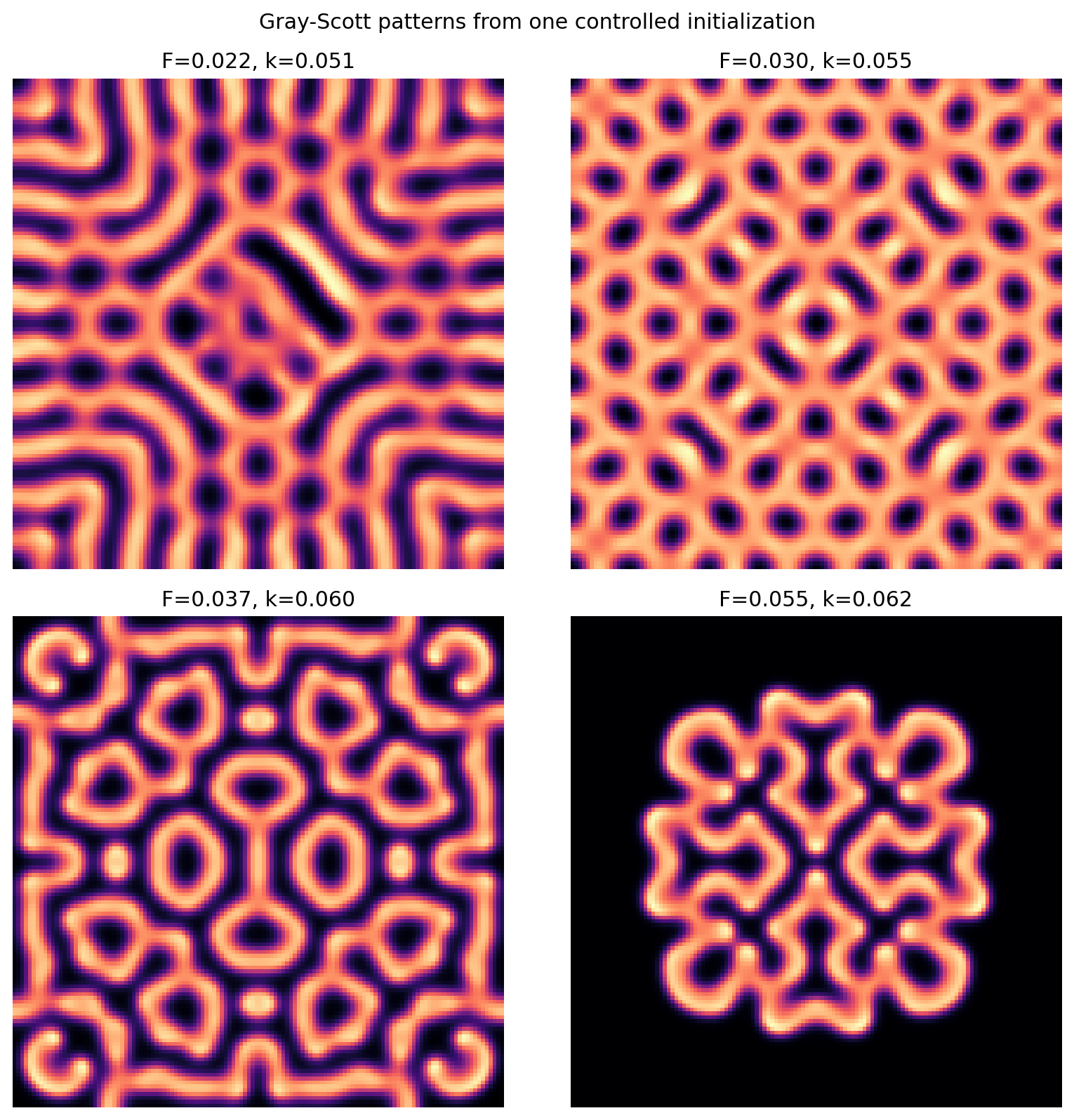
Gray-Scott patterns from controlled feed/kill changes

The point is not merely that the pictures differ.

The point is that small parameter changes move the same local dynamical system into different pattern regimes.

No claim is made here about which set yields spots, stripes, or irregular patterns. Mapping parameter space to pattern taxonomy is Pearson’s systematic program; this chapter’s four-point sweep along a rough diagonal of the feed/kill plane only establishes that different regimes exist and respond to those two parameters.

Keep numerical failure visible

Continuous-state simulations can fail numerically.

Check for invalid values:

def validate_fields(u, v):
    assert np.isfinite(u).all()
    assert np.isfinite(v).all()

Do not silently clip NaN or exploding values and then continue as though the result were meaningful.

If an update becomes unstable, that is evidence about the discretization or parameter choice — the previous chapter’s rate ≤ 1/4 lesson applies here with two diffusion rates and a nonlinear reaction on top.

Pattern formation comes from competition

There is no spot detector.

There is no stripe template.

No cell knows what the final image should look like.

The global structure emerges from competition among:

diffusion
reaction
feed
removal

One mechanism spreads local differences.

Another locally creates or suppresses them.

Persistent structure can appear where those processes balance.

That is an important conceptual step toward continuous artificial-life systems later in the book.

Perturb after the pattern forms

Once a stable-looking pattern appears, damage part of the field:

v[45:75, 45:75] = 0.0
u[45:75, 45:75] = 1.0

Then continue.

Possible outcomes include:

pattern reinvades
new structure forms
damage persists
global state reorganizes

Do not call this regeneration automatically.

At this point it is simply a perturbation-response experiment.

Later, when we train neural cellular automata specifically for recovery, we will define regeneration much more carefully.

Measure more than the mean

Simple statistics:

def field_stats(v):
    return {
        "mean": float(v.mean()),
        "std": float(v.std()),
        "min": float(v.min()),
        "max": float(v.max()),
    }

are useful sanity checks, but very different spatial patterns can share similar means and variances.

Spatial measurements go further. Part III adds spatial variation, entropy and persistence; the others in this list are left for the reader:

connected components
spatial frequency
entropy
persistence
autocorrelation

The image reveals structure.

The measurements let us compare it.

Is Gray-Scott a cellular automaton?

Terminology varies.

A Gray-Scott lattice implementation can also be described as a finite-difference reaction-diffusion simulation or lattice dynamical system.

For this book the architectural continuity is what matters:

discrete spatial lattice
local neighborhood operator
shared local update
repeated time steps

We are extending the same local-computation viewpoint rather than claiming that every lattice PDE discretization belongs to one strict historical CA definition.

One idea to keep

Continuous fields do not remove emergence.

They give local rules more expressive state.

We now have cells that carry multiple interacting quantities and can create persistent spatial structure through local competition.

In the next chapter we will move from chemical fields to a predator-prey ecosystem of local populations and confront a new problem: what happens when multiple agents want to act on the same space?

Research

Pearson, J. E. — Complex Patterns in a Simple System (Science 261, 1993). The provenance for this chapter’s entire experiment: finite-amplitude perturbations of the Gray-Scott autocatalytic model produce a surprising variety of spatiotemporal patterns, with the parameter space systematically mapped. Read it before asserting which feed/kill region yields which regime. https://www.science.org/doi/10.1126/science.261.5118.189
Pearson, J. E. — Complex Patterns in a Simple System (preprint). Freely accessible version of the above for readers without journal access. https://arxiv.org/abs/patt-sol/9304003
Zenil, H. & Martinez, G. J. — Cellular Automata (Scholarpedia). Backs the chapter’s scoping: Turing’s morphogenesis as the classic reaction-diffusion frame, and the distinction between a cellular-automaton analogy and a quantitatively validated approximation — the standard this chapter’s qualitative regime-mapping does not yet claim to meet. http://www.scholarpedia.org/article/Cellular_automata