Activity, Density and Change
A cellular automaton can look busy while doing very little that persists.
It can also look visually quiet while preserving a small moving structure for hundreds of generations.
So we need to separate several properties that are easy to confuse:
occupancy
temporal change
spatial variation
persistence
The first three are owned by the previous chapter — density, change_rate/change_curve (our activity observable), and spatial_variation — and are reused here without redefinition. This chapter adds what they cannot see: whether change persists, where it happens, and how runs end.
Together they form our first useful behavioral fingerprint.
Density measures occupancy — reused
density(state) from the previous chapter answers:
What fraction of the world is active?
Nothing about the definition changes here. The reuse is the point: one owner per observable, referenced rather than restated, so later chapters inherit a single meaning.
What this chapter adds is the discipline of pairing density with change before interpreting either — because density tells us how much state is active, never how it is arranged or whether it is changing.
Activity measures temporal change — reused
Activity is what change_rate/change_curve measure: the fraction of cells that changed since the previous generation. Same function, now used systematically:
activity = 0
    no cell changed

activity ≈ 1
    almost every cell changed

0 < activity < 1
    only part of the world changed
The curve matters more than one final value.
A rule may be highly active early and completely frozen later — which is exactly the gap the next section closes.
Transient activity is not persistent activity
Consider two runs.
Run A
generations 0-30:
    high activity

generations 31-500:
    activity = 0
Run B
generations 0-500:
    moderate activity
Their mean activity could be surprisingly similar over a short experiment.
But dynamically they are very different. (Verified: Rule 30 sustains tail activity ≈ 0.50 while the identity rule holds exactly 0.0 — same metric, opposite dynamics.)
So measure late-run activity separately, reusing the previous chapter’s curve:
import numpy as np


def tail_activity(
    history,
    tail=50,
):
    curve = change_curve(history)

    if len(curve) == 0:
        return 0.0

    return float(
        np.mean(curve[-tail:])
    )
This gives us a simple distinction:
early activity
    -> transient dynamics

tail activity
    -> sustained dynamics
That distinction will become increasingly important when we search rule spaces. It is also window-dependent by construction: the tail length is an observation choice, recorded with the experiment like any other.
Count how often each cell changes
Global activity tells us how much of the world changes.
It does not tell us where the change occurs.
Count transitions at each position:
def cell_change_counts(history):
    return np.sum(
        history[1:] != history[:-1],
        axis=0,
    )
Now each cell gets a value:
0
    never changed

5
    changed five times

100
    changed repeatedly
For an elementary automaton started from one active cell, these counts often reveal the expanding causal region directly. (Verified on a Rule 150 seed: change concentrates in the causal diamond, peaking at 5 changes per cell.)
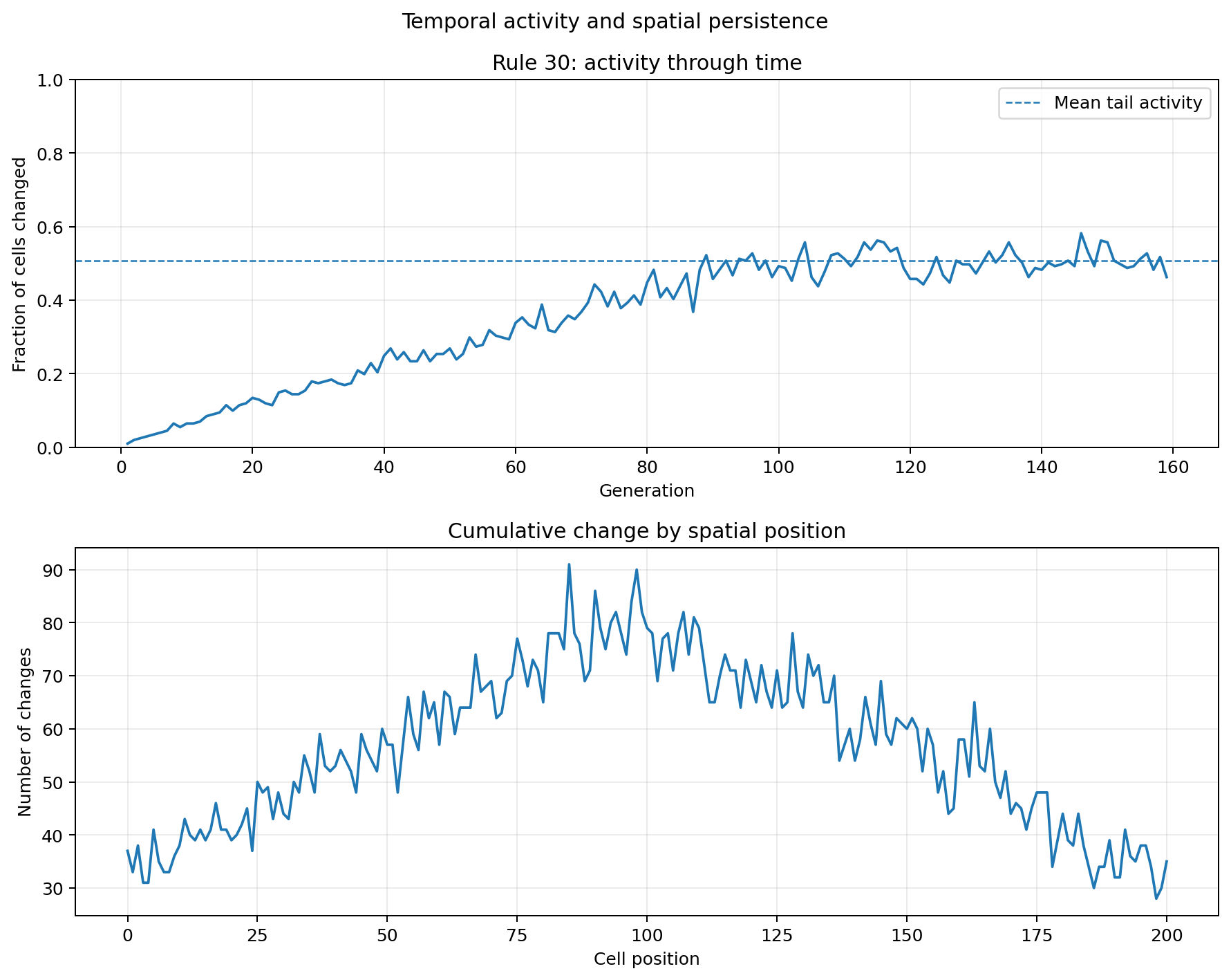
The ordinary spacetime diagram shows the state.
The change-count view shows where dynamics actually occurred.
Detect extinction and saturation explicitly
Binary automata have two particularly simple global states:
all 0
all 1
Detect them directly:
def terminal_state(state):
    if np.all(state == 0):
        return "empty"

    if np.all(state == 1):
        return "full"

    return "mixed"
(Verified: all-zero → “empty”, all-one → “full”, Rule 0 collapses to “empty”.)
This gives search pipelines a cheap first filter.
Rules that immediately become completely empty or full may still be worth understanding, but we do not need expensive measurements to discover that they reached a trivial homogeneous state.
Spatial variation measures local disagreement — reused and extended
spatial_variation(state) from the previous chapter — mean neighbor disagreement — is reused as-is. (Verified: alternating rows score 1.0 while their temporal self-change is 0.0.)
The extension is dimensionality. For a 2D grid:
def spatial_variation_2d(grid):
    horizontal = np.mean(
        grid
        != np.roll(
            grid,
            -1,
            axis=1,
        )
    )

    vertical = np.mean(
        grid
        != np.roll(
            grid,
            -1,
            axis=0,
        )
    )

    return float(
        (horizontal + vertical) / 2
    )
Again, the metric is simple.
It is not a universal measure of structure.
It answers one specific question:
How often do neighboring cells disagree?
That specificity is a strength.
Build a behavioral fingerprint
We now combine the previous chapter’s summary with this chapter’s persistence and terminal observables — extension by composition, not redefinition:
def fingerprint(history):
    return {
        **summarize(history),
        "tail_activity": tail_activity(
            history
        ),
        "terminal": terminal_state(
            history[-1]
        ),
    }
Now a rule does not receive one vague label such as:
complex
It receives a vector of observable properties. (Verified keys: mean/final density, mean change, mean/final spatial variation, tail activity, terminal state.)
The assembly, with each key’s owner:
    flowchart LR
    H[history] --> S[summarize: density, change, spatial]
    H --> T[tail_activity: persistence]
    H --> E[terminal_state: end state]
    S --> F[fingerprint vector]
    T --> F
    E --> F
Component, source, and what can still go wrong:
| Component | Owned helper | Interpretation | Failure mode |
|---|---|---|---|
| mean/final density | summarize (Ch18) | occupancy level | blind to arrangement |
| mean change | summarize (Ch18) | typical turnover | transient-dominated |
| tail activity | tail_activity (here) | sustained dynamics | window-dependent |
| spatial variation | summarize (Ch18) | fragmentation | blind to time |
| terminal state | terminal_state (here) | end regime | says nothing about the route |
Conceptually:
rule
  ↓
trajectory
  ↓
[
    density,
    activity,
    persistence,
    spatial variation,
    terminal behavior
]
That vector can later become input to:
clustering
classification
search
ranking
visualization
Measured on three rules (201 cells, 200 generations, single-cell starts), the vectors are visibly distinct profiles rather than interchangeable scores:
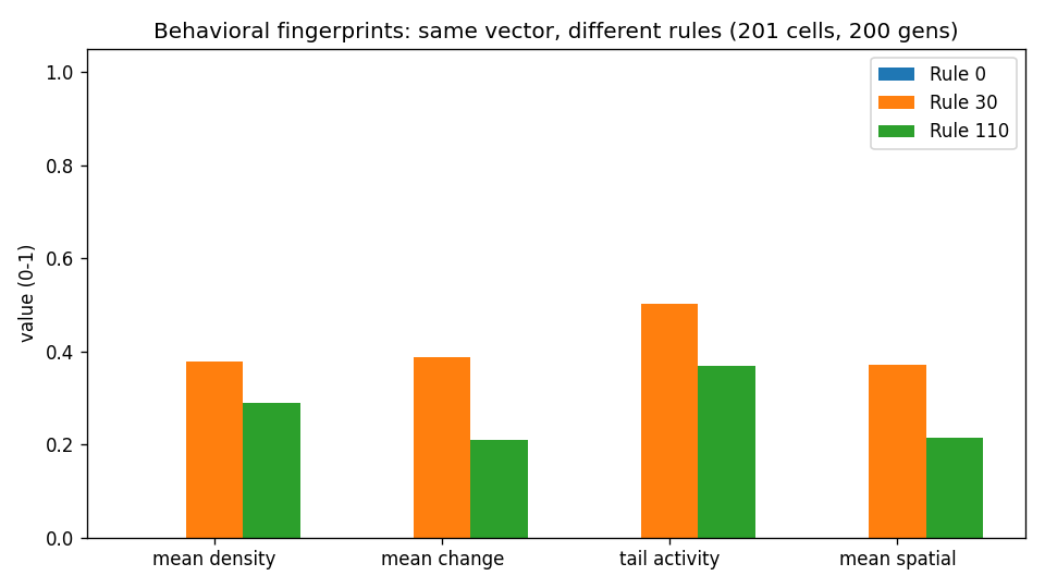
Rule 0 is flat zero everywhere; Rule 30 leads on every axis; Rule 110 sits between, closest on tail activity. The point is not the ranking but the shape: two rules can match on one component and differ sharply on another, which is exactly what a scalar label would hide.
A fingerprint is a measurement vector, not a classification theorem — grouping and labeling rules from these vectors belongs to the classification chapters, which will add their own caveats.
Compare fingerprints, not screenshots
Suppose two rules both look irregular.
Their fingerprints might reveal:
Rule A
mean activity:       high
tail activity:       near zero
spatial variation:   high

Rule B
mean activity:       moderate
tail activity:       moderate
spatial variation:   moderate
Now we know something important.
Rule A creates a violent transient and then settles.
Rule B maintains ongoing dynamics.
A screenshot taken at generation 20 might make them look similar.
A trajectory-level measurement separates them.
Evaluate several initial conditions
A rule is not fully characterized by one initial state.
Run the same rule from several random initial conditions, reusing the previous chapter’s runner — now with the seed and random-initial arguments it was designed for:
def evaluate_rule(
    rule_number,
    seeds,
    width=201,
    generations=200,
):
    records = []

    for seed in seeds:
        history = run_rule(
            rule_number,
            width=width,
            generations=generations,
            seed=seed,
            initial="random",
        )

        records.append(
            fingerprint(history)
        )

    return records
Now calculate:
mean metric value
variance across runs
minimum
maximum
(Verified on Rule 30: five seeds give final densities 0.49–0.54 — stable fingerprint with genuine run-to-run variance.)
A rule whose measurements vary dramatically across initial conditions behaves differently from one whose fingerprint is extremely stable.
Chapter 22 studies that sensitivity directly.
Preserve the experimental context
A fingerprint without context can be misleading.
Record:
rule
initial-condition type
seed
width
generations
boundary condition
measurement version
For example:
record = {
    "rule": 30,
    "initial": "random",
    "seed": 42,
    "width": 201,
    "generations": 200,
    "boundary": "periodic",
    "features": fingerprint(history),
}
Now our feature vector remains tied to the experiment that produced it.
Metrics are features, not truth
A high-activity rule is not automatically interesting.
A low-activity rule is not automatically simple.
A checkerboard has high spatial variation while remaining highly regular.
A transient explosion can produce high mean activity without persistent dynamics.
So the correct pipeline is:
observation
    ↓
measurement
    ↓
comparison
    ↓
hypothesis
    ↓
another experiment
not:
single metric
    ↓
final interpretation
One idea to keep
Density tells us how much state is active. (Owned: Chapter 18.)
Activity tells us how much state is changing. (Owned: Chapter 18; persistence added here.)
Spatial variation tells us how locally fragmented the state is. (Owned: Chapter 18; 2D extension here.)
Persistence tells us whether the dynamics survive. (Owned: this chapter.)
Together they already distinguish systems that a single screenshot or scalar measurement would collapse together.
In the next chapter we will add an information-theoretic observable: Shannon entropy.
It will give us another useful measurement — and another opportunity to learn why a high score does not automatically mean high complexity.
Research
Zenil, H. & Martinez, G. J. — Cellular Automata (Scholarpedia). Supports this chapter’s two methodological moves: finite observations can miss long transients (the reason tail activity exists as a separate observable), and sensitivity/perturbation analysis — Hamming-distance damage spreading and its metric dependence — is the formal sequel to the multi-seed variance measured here. http://www.scholarpedia.org/article/Cellular_automata
Berto, F. & Tagliabue, J. — Cellular Automata (Stanford Encyclopedia of Philosophy). Frames the fingerprint project as an answer to the emergence-detection problem (Miller & Page: is there an objective basis for recognizing emergence?): domains, particles, and intrinsic computation identified through systematic observation rather than visual impression — the tradition this chapter’s vectors join. https://plato.stanford.edu/entries/cellular-automata/