Entropy and Information
A row with almost all zeros is highly predictable.
A row containing a balanced mixture of zeros and ones is less predictable.
Shannon entropy gives us a precise way to measure that uncertainty — defined by Claude Shannon in 1948 as the expected surprise of a distribution, measured here in bits (base 2).
This chapter formally owns what Chapter 3 previewed: the preview binary_entropy becomes the definition below, with the base convention, edge cases, and limitations stated properly.
Binary entropy
If a binary state contains a fraction p of ones, then:
H = -p log2(p) - (1-p) log2(1-p)
In Python:
import math
import numpy as np


def binary_entropy(state):
    p = float(np.mean(state))

    if p in (0.0, 1.0):
        return 0.0

    return -(p * math.log2(p) + (1 - p) * math.log2(1 - p))
The maximum is 1 bit when zeros and ones occur equally often.
(Verified: all-zero → 0.0, all-one → 0.0, exact 50/50 → 1.0, 10% bias → 0.50, random row → 0.99.)
One consequence is easy to miss: binary entropy is a function of density alone. It re-expresses how far p is from 0.5 and sees no arrangement at all, so the row-level entropy curve below adds little beyond the density curve. The neighborhood entropy in the next section is where the observable starts to register spatial structure.
Entropy is not complexity
Consider random coin flips.
They can have nearly maximal entropy.
But random noise has little reusable structure.
So:
high entropy != complex organization
high entropy != intelligence
high entropy != computational universality
low entropy  != simple dynamics
A frozen checkerboard of activity can sit beside a rich glider system at the same entropy. Entropy measures uncertainty in a distribution.
It does not tell us whether patterns persist, interact or compute.
Neighborhood entropy
Instead of counting individual cells, count local patterns.
For a radius-1 elementary automaton, collect neighborhoods of length three:
from collections import Counter


def neighborhood_entropy(state, width=3):
    patterns = []
    n = len(state)

    for i in range(n):
        pattern = tuple(state[(i + j) % n] for j in range(width))
        patterns.append(pattern)

    counts = Counter(patterns)
    total = len(patterns)

    entropy = 0.0
    for count in counts.values():
        p = count / total
        entropy -= p * math.log2(p)

    return entropy
Now we measure diversity of local structures rather than only the global proportion of ones. (Verified: uniform rows → 0.0, alternating rows → 1.0 over two pattern types, random rows → 2.97 against a ceiling of log2(8) = 3.)
Entropy over time
def entropy_curve(history):
    return np.array([binary_entropy(row) for row in history])
Useful questions include:
Does entropy collapse?
Does it remain high?
Does it oscillate?
Does it rise from a simple seed?
That last case is particularly interesting: simple initial conditions producing sustained informational diversity.
Measured across four histories, entropy alone cannot tell noise from Rule 30 — which is precisely the chapter’s thesis made visible:
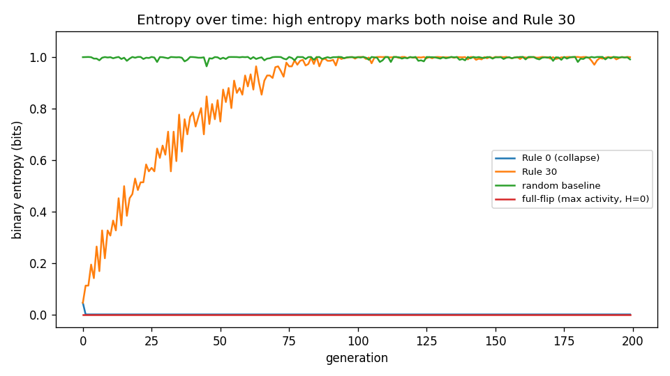
The full-flip world (alternating all-zeros/all-ones, change rate exactly 1.0) holds entropy at zero: maximum activity, minimum uncertainty. Rule 30 and independent random bits are indistinguishable on this axis. High entropy marks both — so whatever distinguishes them must come from the other observables, not from entropy itself. (Verified: Rule 30 from a single cell holds tail entropy ≈ 0.99 over 200 generations.)
Compare entropy with activity
Create a joint record, reusing Chapter 18’s activity observable rather than redefining it:
def information_summary(history):
    entropies = entropy_curve(history)
    activities = change_curve(history)

    return {
        "mean_entropy": float(entropies.mean()),
        "tail_entropy": float(entropies[-50:].mean()),
        "mean_activity": float(activities.mean()),
    }
Rules can now occupy different regions:
low entropy / low activity
high entropy / high activity
high entropy / low activity
moderate entropy / sustained activity
Those regions often correspond to qualitatively different dynamics.
Compression as another lens
Structured data often compresses well.
Random data usually does not.
Python gives us a quick experiment:
import zlib


def compression_ratio(history):
    raw = np.packbits(history.astype(np.uint8)).tobytes()
    compressed = zlib.compress(raw)
    return len(compressed) / len(raw)
This is not a formal complexity measure, but it can expose repeated structure that simple cell entropy misses. Keep three distinct concepts separated:
| Notion | What it measures | What it does not establish |
|---|---|---|
| Shannon entropy | uncertainty of a distribution (exact, given it) | structure, meaning, randomness-as-process |
| compression ratio | upper bound on description length under one compressor | anything compressor-independent; poor compression never proves randomness |
| algorithmic complexity | shortest program producing the object | computability in practice — uncomputable in general |
The interesting middle
A recurring idea in complex systems is that interesting behavior often appears between two extremes:
perfect order <------> random disorder
Cellular automata make that idea visible.
Some rules freeze.
Some become repetitive.
Some look irregular.
A smaller set supports persistent structures and interactions.
Our metrics will help us search that middle rather than selecting purely by eye. Whether that middle is a sharp transition with formal content is a classification question — owned by the chapter that follows the recurrence and sensitivity measurements, not settled here.
Next: repetition
Entropy tells us about uncertainty.
But a system can have a rich-looking state and still repeat exactly every few generations.
The next chapter adds explicit detection of fixed points, cycles and attractors.
Research
Shannon, C. E. — A Mathematical Theory of Communication (Bell System Technical Journal 27, 1948). The definition behind every entropy in this chapter: uncertainty as expected surprise, with the bit as unit. Read the original framing before using entropy as a phenomenon-word — Shannon quantifies a distribution, not a dynamics. https://ieeexplore.ieee.org/document/6773024
Zenil, H. & Martinez, G. J. — Cellular Automata (Scholarpedia). Supplies the chapter’s two guardrails in the literature’s words: entropy characterizes state- or block-frequency distributions (not structure itself), and a compressor gives an upper bound on description length — poor compression by one algorithm is not proof of algorithmic randomness. http://www.scholarpedia.org/article/Cellular_automata