Search All 256 Elementary Rules
Elementary cellular automata give us a rare luxury.
The complete rule space is tiny.
There are only:
256 rules
So we do not need sampling, intuition or famous examples.
We can evaluate every rule.
Build an experiment runner
Reuse the owned helpers with their real signatures — Chapter 18’s runner (rule number, width, generations, seed, single-or-random start) and Chapter 19’s fingerprint:
def scan_rules(width=201, generations=200):
    records = []

    for rule in range(256):
        history = run_rule(
            rule,
            width=width,
            generations=generations,
        )

        record = fingerprint(history)
        record["rule"] = rule
        record["mean_entropy"] = float(
            entropy_curve(history).mean()
        )
        record["compression_ratio"] = compression_ratio(
            history
        )
        record.update(recurrence_metrics(history))

        records.append(record)

    return records
The hard part is no longer execution.
It is deciding what to look for.
Rank by different questions
Most active rules (by the fingerprint’s own activity key):
sorted(records, key=lambda r: r["mean_change"], reverse=True)[:10]
Most persistent:
sorted(records, key=lambda r: r["tail_activity"], reverse=True)[:10]
Most compressible:
sorted(records, key=lambda r: r["compression_ratio"])[:10]
Highest estimated sensitivity — computed for shortlisted candidates only, since each score costs fifty paired runs:
sorted(shortlist, key=lambda r: r["sensitivity"], reverse=True)[:10]
Each ranking answers a different question.
A score is not the phenomenon
Before trusting any ranking, watch one get gamed. A world that flips every cell every generation — all zeros, then all ones, forever — scores the maximum possible mean activity of 1.0 while holding zero entropy and doing nothing anyone would call interesting. (Verified: mean change exactly 1.0, entropy exactly 0.0.)
That is the central warning of search, and it recurs through the rest of the book into learned rules and engineering:
search objective
    = what the system can see

    not necessarily
    = what the author actually cares about

high score
  ≠ good rule
  ≠ meaningful behavior
  ≠ generalization
Defend with region constraints rather than single maxima. Every ranking below is gameable in a specific way — know the exploit before trusting the order:
| Search objective | Metric maximized | Winning exploit | Defense |
|---|---|---|---|
| most active | mean change | full-flip world (1.0, trivial) | require entropy + persistence |
| most persistent | tail activity | frozen near-miss patterns | require nonzero change |
| most compressible | 1 − compression ratio | uniform blank (perfect score) | require activity floor |
| highest entropy | mean entropy | pure noise | require structure measures |
Search for a region, not a maximum
If we maximize entropy alone, we may mostly find noise-like behavior.
Instead define constraints:
candidates = [
    row for row in records
    if 0.35 < row["mean_entropy"] < 0.95
    and row["tail_activity"] > 0.05
    and row["compression_ratio"] < 0.9
]
This searches for a behavioral region rather than a single extreme. (The entropy and compression keys come from the extended record built above — never from the bare fingerprint, which does not contain them.)
Why the filter matters is visible in the distribution itself — measured tail activity across all 256 rules, with the 0.05 cutoff drawn:
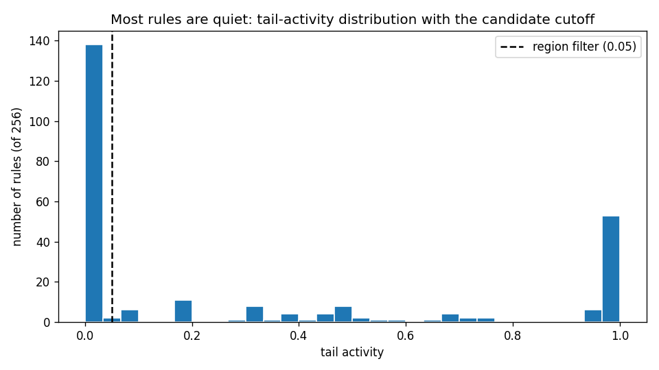
116 of 256 rules clear 0.05; the rest are frozen, dead, or decayed within the window. The cutoff does not discover interestingness — it discards the obviously quiet majority so inspection effort goes where dynamics survive. Note the extreme right bin too: maximum turnover includes trivial full-flip rules, which is why the region filter pairs activity with entropy and compression bounds rather than ranking by it.
Multiple initial conditions
One single-cell experiment strongly favors rules that respond to sparse seeds.
Run several protocols:
single active cell
random density 10%
random density 50%
periodic pattern
structured perturbation
Store a record per (rule, protocol, seed).
Then aggregate by rule.
This prevents one arbitrary setup from becoming the definition of the rule.
Save the catalog
Python’s standard library is enough:
import csv

with open("eca-catalog.csv", "w", newline="") as f:
    writer = csv.DictWriter(f, fieldnames=records[0].keys())
    writer.writeheader()
    writer.writerows(records)
Now rule exploration becomes repeatable data analysis.
Generate contact sheets
Numbers should guide inspection, not eliminate it.
Take the top candidates and render them together:
fig, axes = plt.subplots(4, 4, figsize=(12, 12))

for ax, row in zip(axes.flat, candidates[:16]):
    history = run_rule(row["rule"], width=151, generations=120)
    ax.imshow(history, cmap="binary", interpolation="nearest")
    ax.set_title(f"Rule {row['rule']}")
    ax.axis("off")
The workflow is now — the book’s search loop in its most explicit form:
    flowchart LR
    E[enumerate all 256 rules] --> R[run identical protocol]
    R --> M[measure: fingerprint + entropy + compression]
    M --> F[filter by region, rank within it]
    F --> V[visual inspection of survivors]
    V --> H[hypothesis]
That is much stronger than browsing rules at random — one pipeline from enumeration to hypothesis, with human inspection still in the loop.
Validate famous examples
Our pipeline should rediscover familiar behavioral differences among rules such as 0, 4, 30, 90, 110 and 184.
If it cannot separate obviously different cases, the measurement suite needs work.
Known examples become tests for our instrumentation rather than answers we hard-code.
The luxury disappears quickly
Elementary CA are unusually small.
Increase the neighborhood radius, number of states or dimensions and the number of possible rules explodes.
Then exhaustive search becomes impossible.
The next chapter searches larger rule spaces: what to do when we can no longer evaluate everything.
Research
Wolfram, S. — Statistical Mechanics of Cellular Automata (Reviews of Modern Physics 55, 1983). The original exhaustive scan this chapter replays with modern tooling: all 256 tables run under one protocol and sorted by observed behavior. Reread it as a search paper — protocol, observables, classes — and this chapter is its programmable descendant. https://doi.org/10.1103/RevModPhys.55.601
Zenil, H. & Martinez, G. J. — Cellular Automata (Scholarpedia). The reason the multi-protocol section exists: finite observations miss transients and confuse finite-size effects with system properties, so one setup never defines a rule — plus the rule-table versus trajectory-measure distinction that explains why this chapter searches behavior rather than table patterns. http://www.scholarpedia.org/article/Cellular_automata