Growth Functions
We now have two pieces:
continuous state
      ↓
weighted neighborhood
But a neighborhood value does not tell us what should happen next.
We need a response curve.
In Lenia-style systems that curve is usually called a growth function.
It converts neighborhood potential into local growth or decay. This generalizes Chapter 28’s growth_function: same Gaussian-bump shape, now with explicit mu (preferred density) and sigma (tolerance) parameters instead of fixed constants.
A Gaussian-shaped preference
A useful starting point is:
import numpy as np


def gaussian_growth(u, mu=0.15, sigma=0.03):
    return 2.0 * np.exp(
        -((u - mu) ** 2) / (2 * sigma ** 2)
    ) - 1.0
The output is approximately:
-1   strong decay
 0   neutral
+1   strong growth
(Verified: exactly +1 at u == mu, decaying to −1.0 at both tails.)
Plot it:
import matplotlib.pyplot as plt

u = np.linspace(0.0, 0.4, 500)
g = gaussian_growth(u)

plt.plot(u, g)
plt.axhline(0.0, linewidth=1)
plt.xlabel("neighborhood potential")
plt.ylabel("growth")
plt.show()
The rule prefers a particular local density around mu.
Too little activity decays.
Too much activity also decays.
Only a band around the preferred neighborhood produces positive growth.
Why this can create boundaries
Imagine a blob of active cells.
Inside the blob:
neighborhood potential may be too high
→ decay
Far outside:
neighborhood potential is too low
→ decay
Near a certain boundary region:
neighborhood potential is just right
→ growth
That creates a feedback mechanism capable of maintaining spatial structure.
The rule does not explicitly say:
Make an organism-shaped boundary.
It only rewards a certain local field value — and the guardrail holds: a maintained boundary is a persistent pattern, not an organism.
Growth is not next state
This distinction matters:
growth = gaussian_growth(neighborhood)
is not the next state.
We integrate it:
def integrate(state, growth, dt=0.1):
    return np.clip(state + dt * growth, 0.0, 1.0)
So the full step becomes:
def lenia_like_step(state, kernel, dt=0.1, mu=0.15, sigma=0.03):
    neighborhood = fft_convolve(state, kernel)
    growth = gaussian_growth(neighborhood, mu=mu, sigma=sigma)
    return np.clip(state + dt * growth, 0.0, 1.0)
Perception (fft_convolve, previous chapter), reaction (gaussian_growth, this chapter), integration (dt + clip, Chapter 28) — each owned by exactly one chapter, composed here:
    flowchart LR
    S[state] --> P[perception: convolve kernel]
    P --> G[growth response: gaussian bump]
    G --> I[integrate: state + dt·growth, clip]
    I --> S
Parameters now have clear meanings
We can interpret each parameter — and what happens when it moves:
| Parameter | Role | If increased | If decreased |
|---|---|---|---|
| mu | preferred neighborhood density | prefers crowded contexts | prefers sparse contexts |
| sigma | tolerance around preference | broad, forgiving growth | narrow, selective growth |
| dt | speed of change | faster evolution, instability risk | slower, safer convergence |
| kernel | spatial scale of perception | larger structures sensed | finer local detail |
This is much better than hiding everything inside a single opaque update function.
Narrow versus broad growth
Try:
for sigma in [0.01, 0.03, 0.08]:
    plt.plot(u, gaussian_growth(u, mu=0.15, sigma=sigma), label=str(sigma))

plt.legend(title="sigma")
plt.show()
A narrow function is selective.
A broad function tolerates many neighborhood values — rendered here from the exact function above, no smoothing or artistic license:
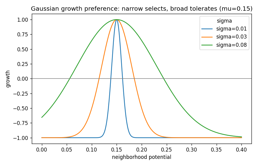
That can radically change the stability of patterns.
Growth fields are worth visualizing
During debugging, show all three layers:
state
neighborhood
local growth
fig, axes = plt.subplots(1, 3, figsize=(12, 4))
axes[0].imshow(state, cmap="viridis")
axes[1].imshow(neighborhood, cmap="magma")
axes[2].imshow(growth, cmap="coolwarm", vmin=-1, vmax=1)
plt.show()
A pattern that mysteriously dies becomes much easier to explain when you can see that almost every cell is receiving negative growth.
Growth and decay balance
A localized pattern survives only if growth and decay balance over time.
Track total mass:
masses = []

for _ in range(500):
    masses.append(state.sum())
    state = lenia_like_step(state, kernel)
Possible outcomes:
mass -> 0
pattern dies

mass -> grid maximum
pattern floods world

mass oscillates in bounded range
persistent dynamics
(Verified over 200 steps from a random seed block: finite throughout, mass in the thousands — neither collapse nor flood on this configuration.)
Persistence does not require exact mass conservation.
It requires long-term balance between local creation and removal.
Later Flow-Lenia will deliberately change this assumption.
Growth curves can be different shapes
A Gaussian is convenient, not mandatory.
For example:
def triangular_growth(u, center=0.15, width=0.05):
    score = 1.0 - np.abs(u - center) / width
    return np.clip(2 * score - 1, -1, 1)
(Verified: +1 at center, −1 at both edges of the support.)
Or a smooth polynomial bump.
Different response families create different dynamical systems.
Inspect local causality
Pick one cell:
y, x = 64, 64

print("state:", state[y, x])
print("neighborhood:", neighborhood[y, x])
print("growth:", growth[y, x])
This gives a local causal chain:
surrounding state
      ↓
weighted perception
      ↓
growth response
      ↓
state increment
Even when the global pattern becomes astonishingly complex, the local mechanism remains inspectable.
We now have almost all of Lenia’s skeleton
At the highest level:
A(t)
  ↓ convolution K
U(t)
  ↓ growth G
G(U)
  ↓ small integration step
A(t + dt)
The next chapter will put those components together into a reusable implementation.
We will not begin by copying a mysterious Lenia codebase.
We will build Lenia from first principles, component by component, using the machinery we already understand.
Research
Zenil, H. & Martinez, G. J. — Cellular Automata (Scholarpedia). The continuous-variants context for the whole skeleton: discrete-space, discrete-time systems with continuous states are legitimate extensions outside the strict finite-state definition — the status every component assembled here carries. http://www.scholarpedia.org/article/Cellular_automata
Berto, F. & Tagliabue, J. — Cellular Automata (Stanford Encyclopedia of Philosophy). The emergence framing this chapter earns rather than assumes: complex global behavior from simple local rules is the observed phenomenon under study, with the growth/decay balance as its continuous-state mechanism — interpretation layered on measurement, not substituted for it. https://plato.stanford.edu/entries/cellular-automata/