Measure a Cellular Automaton
Up to this point we have mostly looked at cellular automata.
That is useful.
It is also limiting. Part II closed by asking how we tell which worlds are dynamically interesting, and looking cannot answer that at scale.
A human can inspect a handful of spacetime diagrams.
We cannot reliably inspect:
256 elementary rules
× several initial conditions
× several widths
× hundreds of generations
× repeated stochastic runs
by eye.
If we want to compare rules, search for interesting behavior or eventually optimize a rule for some objective, we need to turn behavior into data.
This chapter builds the measurement layer.
One vocabulary note before the definitions: Chapter 3 previewed lightweight curve helpers on whole histories. Those were forerunners. Here each observable gets a formal owner — a per-state or per-pair definition first, lifted to curves second — and the next chapter reuses them without redefining them.
A second orientation note: there are two families of measures in this field. Rule-table measures (Langton’s λ is the classic example: the fraction of table entries leading away from quiescence) are computed without running anything, but they do not uniquely determine the dynamics. Trajectory measures — everything in this chapter — are computed from observed evolution, but they can miss long transients and confuse finite-size effects with infinite-system properties. We work in the second family with the first family’s limitation in mind.
A simulation produces a trajectory
For a one-dimensional binary cellular automaton, a complete run can be stored as:
history.shape
# (generations, cells)
Every row is one state of the world.
So:
history[t]
means:
the complete spatial state at generation t
The matrix is not merely something to plot.
It is a dataset.
We can ask:
How many cells are active?

How much changes between generations?

How fragmented is the spatial pattern?

Does the system become fixed?

Does it repeat?

How sensitive is it to initial conditions?
No single answer defines complexity.
But each answer exposes one observable property of the dynamics.
To ask these questions reproducibly we need one runnable helper, used here and reused by the next chapters — a rule runner with explicit initial-condition control:
def run_rule(
    rule_number,
    width=201,
    generations=200,
    seed=None,
    initial="single",
):
    if initial == "random":
        rng = np.random.default_rng(seed)
        state = (rng.random(width) < 0.5).astype(np.uint8)
    else:
        state = np.zeros(width, dtype=np.uint8)
        state[width // 2] = 1

    history = [state.copy()]

    for _ in range(generations - 1):
        state = step(state, rule_number)
        history.append(state.copy())

    return np.array(history)
It uses Chapter 3’s step (periodic ring) and returns the array-valued history the whole book shares.
Density
The simplest measurement is the fraction of active cells:
import numpy as np


def density(state):
    return float(np.mean(state))
For:
00011101
four of eight cells are active:
density = 0.5
(Verified across the battery: all-zero → 0.0, all-one → 1.0, alternating → 0.5.)
Across an entire run:
def density_curve(history):
    return np.mean(history, axis=1)
Now we have:
generation -> active-cell fraction
Different systems can behave very differently.
A rule may:
die out
    -> density approaches 0

saturate
    -> density approaches 1

remain mixed
    -> density stays between the extremes

oscillate
    -> density changes periodically
But density alone does not tell us whether the cells are actually changing.
Change rate
Two generations can have exactly the same density while containing active cells in completely different positions.
So measure temporal change directly. This is the book’s activity observable — the fraction changed between successive states:
def change_rate(previous, current):
    return float(
        np.mean(previous != current)
    )
Across a run:
def change_curve(history):
    return np.mean(
        history[1:] != history[:-1],
        axis=1,
    )
Now:
change rate = 0
means the state is unchanged from the previous generation.
A fixed point has:
density = constant
change  = 0
But an oscillator may have:
density = constant
change  > 0
(Verified: Rule 204, the identity rule, holds tail change at exactly 0.0; period-2 alternating rows change at 1.0 — every cell flips.)
That distinction is exactly why we need more than one observable.
Spatial variation
Temporal change tells us what happens between generations.
We can also measure structure inside one generation.
Count how often neighboring cells differ:
def spatial_variation(state):
    right = np.roll(state, -1)

    return float(
        np.mean(state != right)
    )
Compare:
0000000011111111
with:
0101010101010101
Both contain equal numbers of zeros and ones.
So both have:
density = 0.5
But their spatial organization is completely different.
The first has only a few boundaries.
The second changes almost every cell. (Verified: alternating rows score spatial variation 1.0 with temporal self-change 0.0 — the canonical dissociation of space from time.)
Spatial variation gives us a crude measure of local spatial fragmentation: one specific question (“how often do neighboring cells disagree?”), not a general structure score.
The same system needs several views
Consider three questions:
How much is active?
    -> density

How much changes over time?
    -> change rate (activity)

How rough is the spatial arrangement?
    -> spatial variation
These are different properties — owned here, each with a stated blind spot:
| Observable | Definition | Captures | Misses |
|---|---|---|---|
| density | fraction of active cells | occupancy level | arrangement, change |
| change rate (activity) | fraction changed since last step | temporal dynamics | spatial structure |
| spatial variation | fraction of disagreeing neighbors | local fragmentation | temporal dynamics |
That is the key lesson of this chapter — and the guardrail that travels with every metric in the book: density ≠ structure, activity ≠ complexity, and no single curve tells the full story.
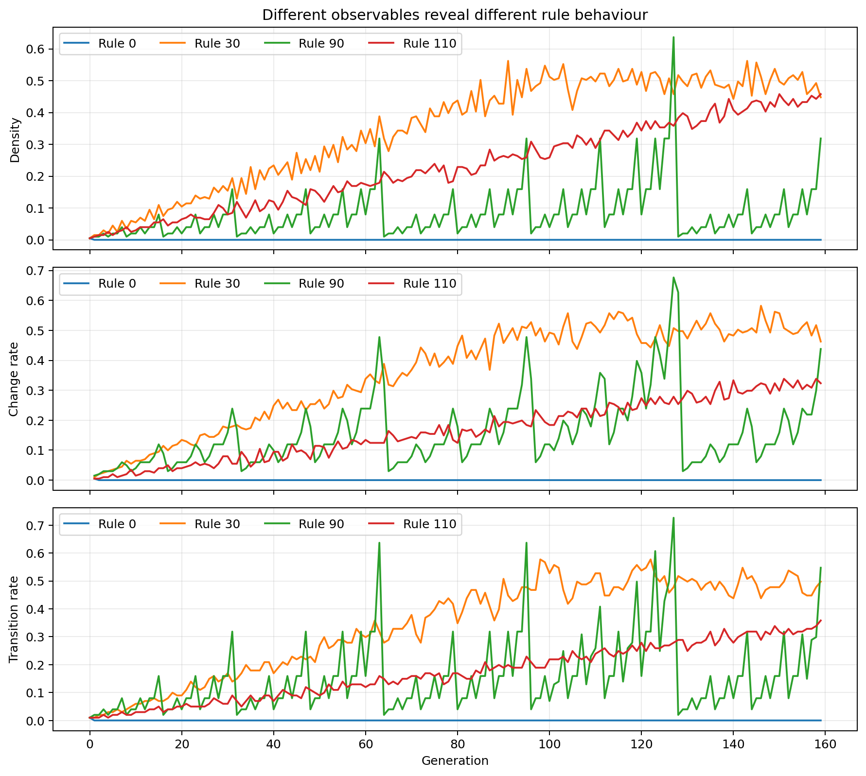
The figure compares several rules from the same initial-condition protocol.
No single curve tells the full story.
Together they begin to form a behavioral fingerprint.
Summarize one run
We can combine basic measurements:
def summarize(history):
    changes = change_curve(history)

    spatial = np.array([
        spatial_variation(state)
        for state in history
    ])

    return {
        "final_density": float(
            density(history[-1])
        ),
        "mean_density": float(
            np.mean(history)
        ),
        "mean_change": float(
            np.mean(changes)
        ) if len(changes) else 0.0,
        "mean_spatial": float(
            np.mean(spatial)
        ),
        "final_spatial": float(
            spatial[-1]
        ),
    }
(Verified: Rule 0 collapses to all zeros on every key; Rule 30 sustains mean change ≈ 0.39.)
Now a trajectory has a compact numerical description.
But that description is only meaningful if we also know how the trajectory was generated.
A measurement without experiment context is incomplete
Rule 30 started from a single active cell is not the same experiment as Rule 30 started from random noise.
Likewise:
periodic boundaries
and:
fixed boundaries
can produce different trajectories.
So a measurement record should include its experimental context.
For example:
result = {
    "rule": 30,
    "width": 201,
    "generations": 200,
    "initial_condition": "single",
    "boundary": "periodic",
    "seed": None,
    "metrics": summarize(history),
}
For a stochastic run we might instead record:
"seed": 42
The rule is:
Never separate a metric from the experiment that produced it.
Turn every rule into a record
Now evaluate all elementary cellular automata:
records = []

for rule_number in range(256):
    history = run_rule(
        rule_number,
        width=201,
        generations=200,
    )

    records.append({
        "rule": rule_number,
        **summarize(history),
    })
We have transformed:
256 images
into:
256 structured records
Now we can sort:
most_active = sorted(
    records,
    key=lambda row: row["mean_change"],
    reverse=True,
)
Filter:
candidates = [
    row
    for row in records
    if 0.2 < row["mean_density"] < 0.8
    and row["mean_change"] > 0.1
]
Or plot rules in measurement space.
This is the beginning of automated exploration.
Preserve trajectories and summaries separately
The summary is convenient.
The trajectory is evidence.
Do not throw away the complete history simply because you calculated a few metrics.
A useful experimental record has two levels:
raw trajectory
      ↓
derived measurements
If a metric later turns out to be misleading, we can calculate a better one from the original run.
That is much harder if only the summary survived.
One metric is never enough
A checkerboard has:
high spatial variation
but it is extremely regular.
Random noise can have:
high entropy
without having persistent structure — with entropy itself defined properly in Chapter 20, not as a synonym for complexity.
An oscillator can have:
high temporal activity
while remaining perfectly predictable.
So we are not searching for:
the complexity number
There probably is no single scalar that captures everything we care about.
Instead we are building a collection of observables — owned here, extended next chapter:
density            (this chapter)
activity           (this chapter: change_rate/change_curve)
spatial variation  (this chapter)
entropy            (Chapter 20)
periodicity        (Chapter 21)
attractor structure(Chapter 21)
sensitivity        (Chapter 22)
persistence        (next chapter: tail activity)
Different questions require different measurements.
The measurement pipeline
We now have a new architecture — the same pipeline as a diagram, for reuse across Part III:
    flowchart LR
    C[experiment configuration] --> S[simulation]
    S --> T[trajectory]
    T --> M[measurements: density, change, spatial]
    M --> R[result record]
    R --> N[next: compare, classify, search]
The next stages will add:
comparison
classification
search
selection
This changes the role of the cellular automaton.
It is no longer only something we render.
It becomes something we can experiment on systematically.
One idea to keep
A measurement does not explain a cellular automaton. (Metric ≠ phenomenon ≠ explanation.)
It gives us another way to interrogate it.
The strongest workflow is:
look
    ↓
measure
    ↓
compare
    ↓
form hypothesis
    ↓
run another experiment
In the next chapter we will reuse these three observables without redefining them, and add what they cannot see: whether change persists, where it happens, and how runs end.
Research
Zenil, H. & Martinez, G. J. — Cellular Automata (Scholarpedia). The methodology backing for this chapter’s two hardest-won points: rule-table measures (Langton’s λ) do not uniquely determine dynamics, so trajectory measurement is necessary — and finite observations can miss long transients and confuse finite-size effects with infinite-system properties, so windows and lattice sizes belong in every record. http://www.scholarpedia.org/article/Cellular_automata
Berto, F. & Tagliabue, J. — Cellular Automata (Stanford Encyclopedia of Philosophy). Frames this chapter’s pipeline as phenomenological study in the literature’s sense: registering emergent properties by running the system, where universal systems admit no shortcut around simulation (Ilachinski; Wolfram’s algorithmic irreducibility) — the reason measurement replaces armchair prediction here. https://plato.stanford.edu/entries/cellular-automata/